import torch
import torch.nn as nn
import torch.nn.functional as F
from sklearn.model_selection import train_test_split
from sklearn.datasets import make_blobs
from latex import latexify
import numpy as np
import matplotlib.pyplot as plt
import matplotlib.patches as mpatches
%matplotlib inline
%config InlineBackend.figure_format = "retina"

if (torch.cuda.is_available()):
    device = torch.device("cuda")
else:
    device = torch.device("cpu")
print(device)

cpu

def generate_xor_dataset(size):
    centers = [[-3.5, 3.5], [-3.5, -3.5], [3.5, -3.5], [3.5, 3.5]]
    X, _ = make_blobs(n_samples = size, centers = centers, n_features = 2, random_state = 13, cluster_std = 2)
    X = torch.FloatTensor(X)
    y = (X[:, 0] > 0) ^ (X[:, 1] > 0)
    return X, y.float().view(-1, 1)

Plotting the XOR Dataset

X, y = generate_xor_dataset(400)
X_train, X_test, y_train, y_test = train_test_split(X, y, test_size = 0.5, random_state = 42)
latexify(columns = 2, fig_width = 7)
plt.scatter(X_train[:, 0], X_train[:, 1], c = y_train, cmap = "viridis", s = 10, label = "Training Samples")
plt.scatter(X_test[:, 0], X_test[:, 1], c = y_test, cmap = "viridis", s = 10, label = "Test Samples", alpha = 0.5)
plt.xlabel(r"$x_1$")
plt.ylabel(r"$x_2$")
plt.title("XOR Dataset - Training and Testing Samples")
plt.legend()
plt.show()

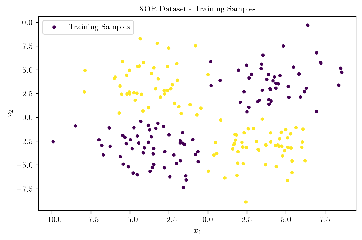
plt.scatter(X_train[:, 0], X_train[:, 1], c = y_train, cmap = "viridis", s = 10, label = "Training Samples")
plt.xlabel(r"$x_1$")
plt.ylabel(r"$x_2$")
plt.title("XOR Dataset - Training Samples")
plt.legend()
plt.show()


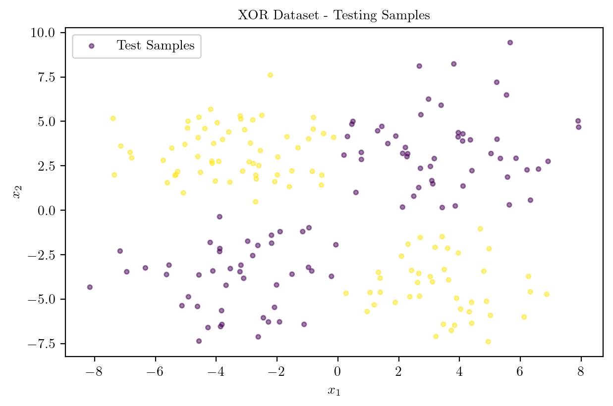
plt.scatter(X_test[:, 0], X_test[:, 1], c = y_test, cmap = "viridis", s = 10, label = "Test Samples", alpha = 0.5)
plt.xlabel(r"$x_1$")
plt.ylabel(r"$x_2$")
plt.title("XOR Dataset - Testing Samples")
plt.legend()
plt.show()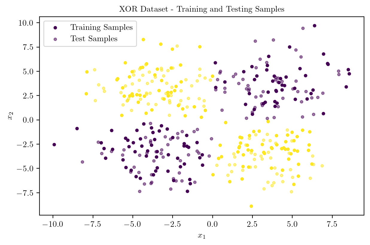

X_train.shape, X_test.shape, y_train.shape, y_test.shape

(torch.Size([200, 2]),
 torch.Size([200, 2]),
 torch.Size([200, 1]),
 torch.Size([200, 1]))

X_train = X_train.to(device)
X_test = X_test.to(device)
y_train = y_train.to(device)
y_test = y_test.to(device)

Model Architecture

class XORMLP(nn.Module):
  def __init__(self, hidden_layer1, hidden_layer2):
    super().__init__()
    self.lin1 = nn.Linear(2, hidden_layer1)
    self.lin2 = nn.Linear(hidden_layer1, hidden_layer2)
    self.lin3 = nn.Linear(hidden_layer2, 1)

  def forward(self, x):
    x = torch.relu(self.lin1(x))
    x = torch.relu(self.lin2(x))
    logits = self.lin3(x)
    return logits

\[\text{Hidden Layer 1} = 3\]

\[\text{Hidden Layer 2} = 2\]

model = XORMLP(hidden_layer1 = 3, hidden_layer2 = 2)

for param_name, param in model.named_parameters():
    print(param_name, param.shape)

lin1.weight torch.Size([3, 2])
lin1.bias torch.Size([3])
lin2.weight torch.Size([2, 3])
lin2.bias torch.Size([2])
lin3.weight torch.Size([1, 2])
lin3.bias torch.Size([1])

model.state_dict()

OrderedDict([('lin1.weight',
              tensor([[ 0.0173,  0.1983],
                      [-0.6344, -0.0252],
                      [ 0.6104,  0.4044]])),
             ('lin1.bias', tensor([ 0.2710, -0.2886,  0.3233])),
             ('lin2.weight',
              tensor([[ 0.1575, -0.3338,  0.0382],
                      [ 0.4192, -0.2178, -0.0236]])),
             ('lin2.bias', tensor([0.1116, 0.5393])),
             ('lin3.weight', tensor([[-0.4375,  0.2778]])),
             ('lin3.bias', tensor([0.6558]))])

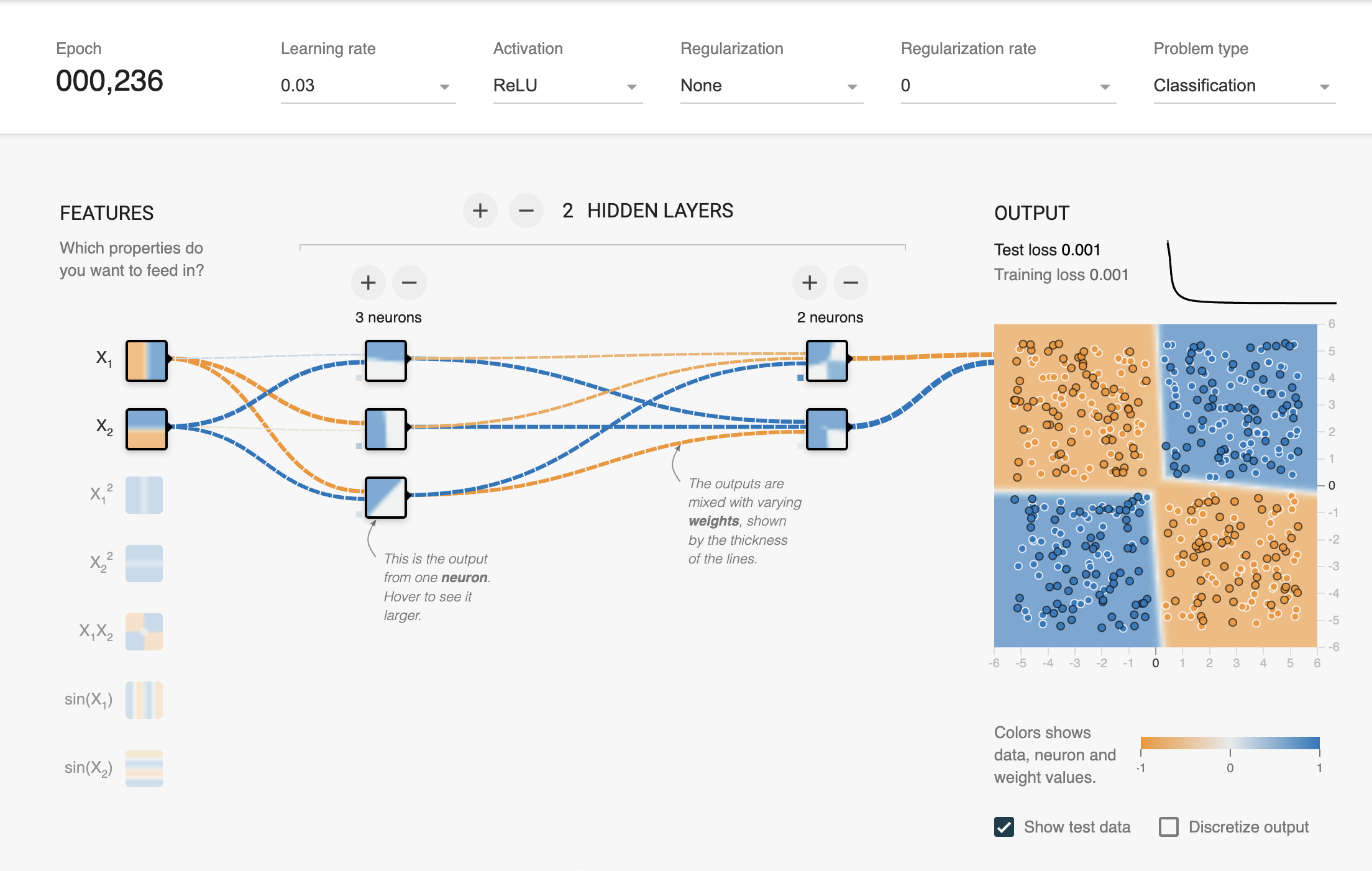
Model Training with NO REGULARIZATION

\[\text{Loss Function} = \text{Binary Cross Entropy with Logits} \] \[L_N = - [y_N \cdot \log({\sigma(\hat{y}_N)}) + (1 - y_N) \cdot \log({1 - \sigma(\hat{y}_N)})]\] \[ \sigma(z) = \frac{1}{1 + e^{-z}}\]

loss_fn = nn.BCEWithLogitsLoss()
optimizer = torch.optim.Adam(model.parameters(), lr = 0.03)

train_dataset = torch.utils.data.TensorDataset(X_train, y_train)
train_loader = torch.utils.data.DataLoader(train_dataset, batch_size = 32, shuffle = True)

for epoch in range(10000):
    running_loss = 0.0
    correct = 0
    total = 0
    for inputs, labels in train_loader:
        optimizer.zero_grad()
        logits = model(inputs)
        loss = loss_fn(logits, labels)
        loss.backward()
        optimizer.step()
        
        running_loss += loss.item()
        correct += ((logits > 0) == labels).sum().item()
        total += labels.size(0)
    
    epoch_loss = running_loss / len(train_loader)
    accuracy = correct / total
    if (epoch + 1) % 1000 == 0:
        print(f"Epoch [{epoch + 1}/10000] | Loss: {epoch_loss} | Accuracy: {accuracy:.7f}")

Epoch [1000/10000] | Loss: 6.0668761372133826e-05 | Accuracy: 1.0000000

KeyboardInterrupt:

Inference from the Model on Training Samples

model.eval()

with torch.no_grad():
    logits = model(X_test)
    predictions = (logits > 0).float()
    accuracy = (predictions == y_test).sum().item() / y_test.size(0)
    print(f"Test Accuracy: {accuracy:.7f}")

Test Accuracy: 0.9800000

Plotting the Decision Surface

def plot_decision_boundary(X_train, X_test, y_train, y_test, model, title):
    X = torch.cat([X_train, X_test], dim = 0).cpu().numpy()
    y = torch.cat([y_train, y_test], dim = 0).cpu().numpy()
    
    x_min, x_max = X[:, 0].min() - 1, X[:, 0].max() + 1
    y_min, y_max = X[:, 1].min() - 1, X[:, 1].max() + 1
    
    xx, yy = np.meshgrid(np.arange(x_min, x_max, 0.1), np.arange(y_min, y_max, 0.1))
    Z = model(torch.FloatTensor(np.c_[xx.ravel(), yy.ravel()]).to(device))
    
    Z = (Z > 0).float().cpu().numpy().reshape(xx.shape)
    
    plt.contourf(xx, yy, Z, cmap = plt.cm.Paired, alpha = 0.4)
    
    plt.scatter(X_train[:, 0], X_train[:, 1], c = y_train, cmap = "viridis", s = 10)
    plt.scatter(X_test[:, 0], X_test[:, 1], c = y_test, cmap = "viridis", s = 10, alpha = 0.5)
    
    yellow_patch = mpatches.Patch(color = "yellow", label = "Class 1")
    blue_patch = mpatches.Patch(color = "darkblue", label = "Class 2")
    pink_patch = mpatches.Patch(color = "darksalmon", label = "Predict Class 1")
    lblue_patch = mpatches.Patch(color = "lightblue", label = "Predict Class 2")
    plt.legend(handles = [yellow_patch, blue_patch, pink_patch, lblue_patch], loc = "upper center", bbox_to_anchor = (0.5, 1.25), ncol = 2, fancybox = True, shadow = True)
    
    plt.title(title)
    plt.xlabel(r"$x_1$")
    plt.ylabel(r"$x_2$")
    plt.show()

Decision Boundary before training

latexify(columns = 2, fig_width = 9)
model = XORMLP(hidden_layer1 = 3, hidden_layer2 = 2)
plot_decision_boundary(X_train, X_test, y_train, y_test, model, "XOR Dataset - Decision Boundary - Untrained MLP")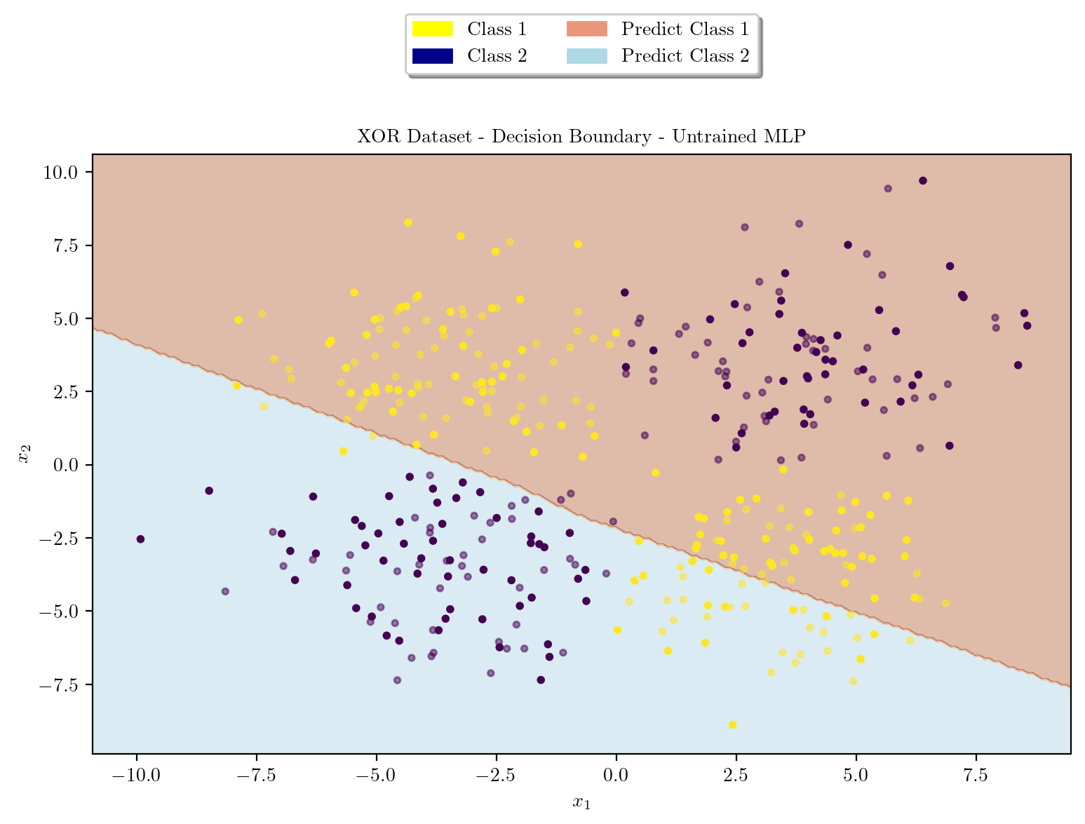

Decision Boundary After Training

latexify(columns = 2, fig_width = 9)
plot_decision_boundary(X_train, X_test, y_train, y_test, model, "XOR Dataset - Decision Boundary - MLP with No Regularization")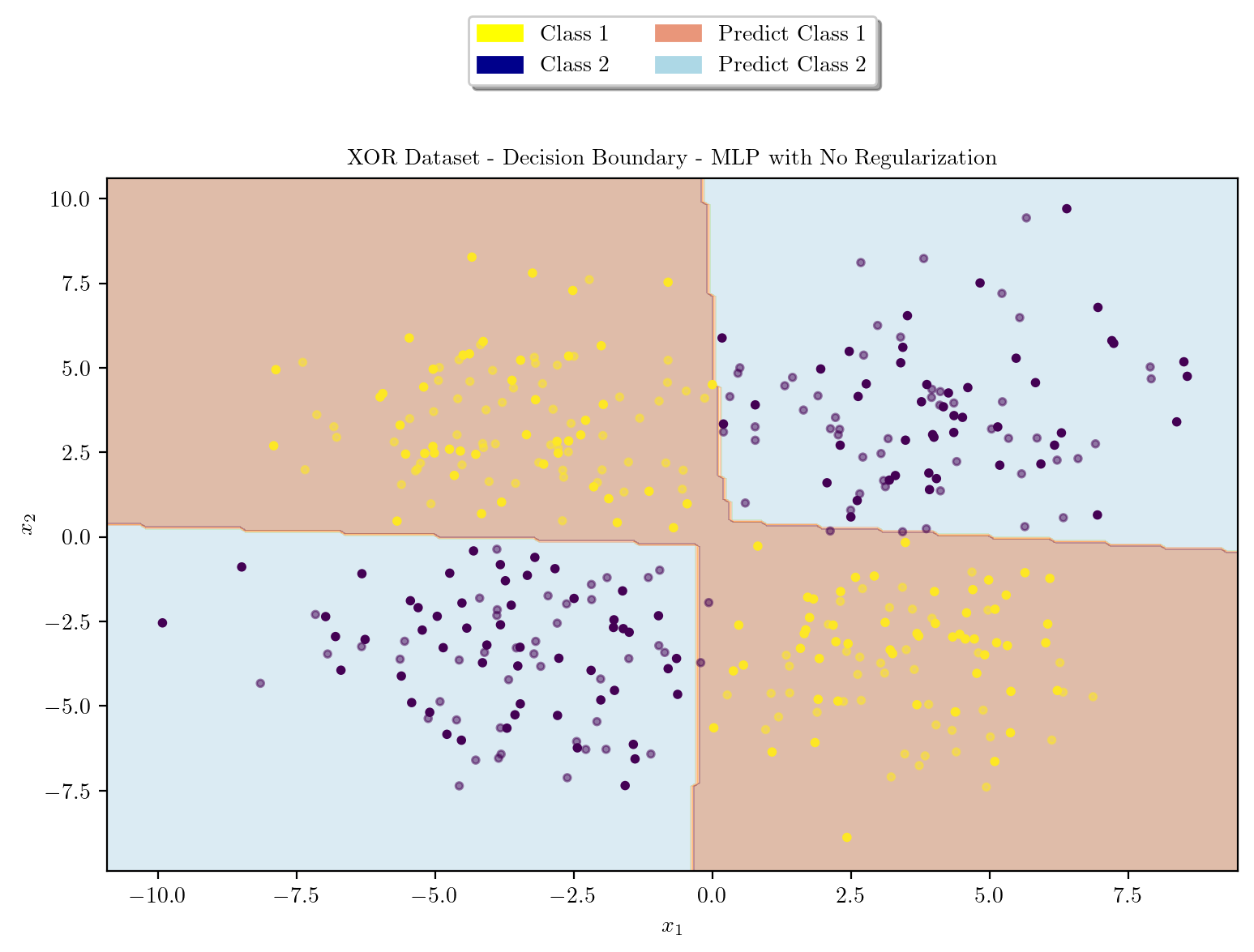

Model Architecture \(L_1\) regularization

\[\text{Hidden Layer 1} = 3\]

\[\text{Hidden Layer 2} = 2\]

model = XORMLP(hidden_layer1 = 3, hidden_layer2 = 2)

for param_name, param in model.named_parameters():
    print(param_name, param.shape)

lin1.weight torch.Size([3, 2])
lin1.bias torch.Size([3])
lin2.weight torch.Size([2, 3])
lin2.bias torch.Size([2])
lin3.weight torch.Size([1, 2])
lin3.bias torch.Size([1])

model.state_dict()

OrderedDict([('lin1.weight',
              tensor([[-0.5916, -0.1956],
                      [-0.6127, -0.6096],
                      [-0.0030, -0.4923]])),
             ('lin1.bias', tensor([-0.2103, -0.3799,  0.0432])),
             ('lin2.weight',
              tensor([[-0.3961, -0.5236, -0.2789],
                      [-0.3070, -0.1840,  0.1793]])),
             ('lin2.bias', tensor([ 0.1382, -0.3959])),
             ('lin3.weight', tensor([[-0.7065, -0.0468]])),
             ('lin3.bias', tensor([-0.2404]))])

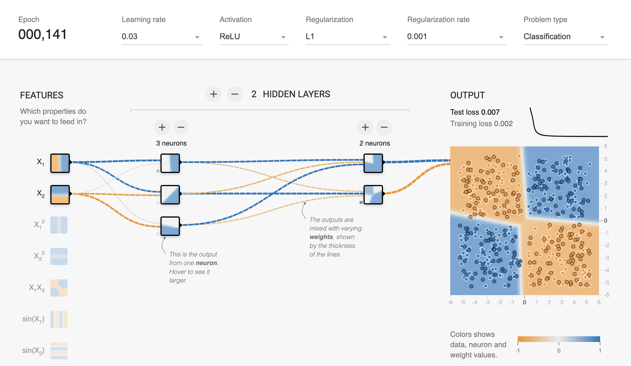
Model Training with \(L_1\) Regularization

\[\text{Loss Function} = \text{Binary Cross Entropy with Logits} + \beta \cdot \sum_{i} ||w_i^T w_i||_1\] \[L_N = - [y_N \cdot \log({\sigma(\hat{y}_N)}) + (1 - y_N) \cdot \log({1 - \sigma(\hat{y}_N)})] + \beta \cdot \sum_{i} ||w_i^T w_i||_1\] \[ \sigma(z) = \frac{1}{1 + e^{-z}}\]

loss_fn = nn.BCEWithLogitsLoss()
optimizer = torch.optim.Adam(model.parameters(), lr = 0.03)

# L1 Regularization Penalty Coefficient
beta = 0.001

train_dataset = torch.utils.data.TensorDataset(X_train, y_train)
train_loader = torch.utils.data.DataLoader(train_dataset, batch_size = 32, shuffle = True)

for epoch in range(10000):
    running_loss = 0.0
    correct = 0
    total = 0
    for inputs, labels in train_loader:
        optimizer.zero_grad()
        logits = model(inputs)
        loss = loss_fn(logits, labels)
        
        l1_regularization = 0.0
        for param in model.parameters():
            l1_regularization += torch.norm(param, 1)
        loss += beta * l1_regularization
        
        
        loss.backward()
        optimizer.step()
        
        running_loss += loss.item()
        correct += ((logits > 0) == labels).sum().item()
        total += labels.size(0)
    
    epoch_loss = running_loss / len(train_loader)
    accuracy = correct / total
    if (epoch + 1) % 1000 == 0:
        print(f"Epoch [{epoch + 1}/10000] | Loss: {epoch_loss} | Accuracy: {accuracy:.7f}")

Epoch [1000/10000] | Loss: 0.0748444204883916 | Accuracy: 0.9900000

KeyboardInterrupt:

model.eval()

with torch.no_grad():
    logits = model(X_test)
    predictions = (logits > 0).float()
    accuracy = (predictions == y_test).sum().item() / y_test.size(0)
    print(f"Test Accuracy: {accuracy:.7f}")

Test Accuracy: 0.9900000

latexify(columns = 2, fig_width = 9)
model = XORMLP(hidden_layer1 = 3, hidden_layer2 = 2)
plot_decision_boundary(X_train, X_test, y_train, y_test, model, "XOR Dataset - Decision Boundary - Untrained MLP")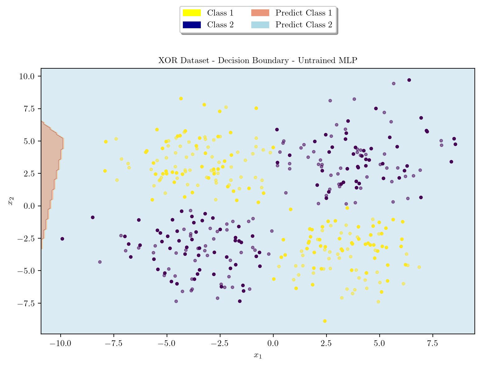

latexify(columns = 2, fig_width = 9)
plot_decision_boundary(X_train, X_test, y_train, y_test, model, r"XOR Dataset - Decision Boundary - MLP with $L_1$ Regularization")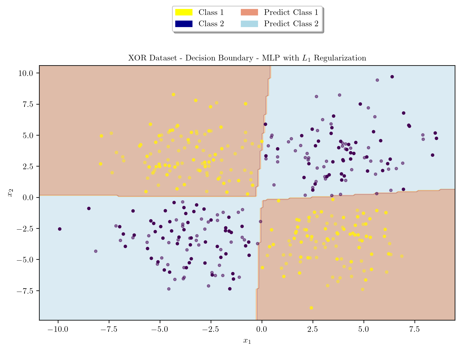

Model Architecture \(L_2\) regularization

\[\text{Hidden Layer 1} = 3\]

\[\text{Hidden Layer 2} = 2\]

model = XORMLP(hidden_layer1 = 3, hidden_layer2 = 2)

for param_name, param in model.named_parameters():
    print(param_name, param.shape)

lin1.weight torch.Size([3, 2])
lin1.bias torch.Size([3])
lin2.weight torch.Size([2, 3])
lin2.bias torch.Size([2])
lin3.weight torch.Size([1, 2])
lin3.bias torch.Size([1])

model.state_dict()

OrderedDict([('lin1.weight',
              tensor([[-0.2630,  0.0580],
                      [ 0.1551,  0.1032],
                      [ 0.2098, -0.4817]])),
             ('lin1.bias', tensor([ 0.0032, -0.6091,  0.0220])),
             ('lin2.weight',
              tensor([[-0.2524,  0.4557,  0.5474],
                      [ 0.3153,  0.3795, -0.3605]])),
             ('lin2.bias', tensor([-0.2719, -0.4453])),
             ('lin3.weight', tensor([[-0.5590, -0.4162]])),
             ('lin3.bias', tensor([-0.6296]))])

Model Training with \(L_2\) Regularization

\[\text{Loss Function} = \text{Binary Cross Entropy with Logits} + \beta \cdot \sum_{i} ||w_i^T w_i||_2\] \[L_N = - [y_N \cdot \log({\sigma(\hat{y}_N)}) + (1 - y_N) \cdot \log({1 - \sigma(\hat{y}_N)})] + \beta \cdot \sum_{i} ||w_i^T w_i||_2\] \[ \sigma(z) = \frac{1}{1 + e^{-z}}\]

loss_fn = nn.BCEWithLogitsLoss()
optimizer = torch.optim.Adam(model.parameters(), lr = 0.03)

# L2 Regularization Penalty Coefficient
beta = 0.001

train_dataset = torch.utils.data.TensorDataset(X_train, y_train)
train_loader = torch.utils.data.DataLoader(train_dataset, batch_size = 32, shuffle = True)

for epoch in range(10000):
    running_loss = 0.0
    correct = 0
    total = 0
    for inputs, labels in train_loader:
        optimizer.zero_grad()
        logits = model(inputs)
        loss = loss_fn(logits, labels)
        
        l1_regularization = 0.0
        for param in model.parameters():
            l1_regularization += torch.norm(param, 2)
        loss += beta * l1_regularization
        
        loss.backward()
        optimizer.step()
        
        running_loss += loss.item()
        correct += ((logits > 0) == labels).sum().item()
        total += labels.size(0)
    
    epoch_loss = running_loss / len(train_loader)
    accuracy = correct / total
    if (epoch + 1) % 1000 == 0:
        print(f"Epoch [{epoch + 1}/10000] | Loss: {epoch_loss} | Accuracy: {accuracy:.7f}")

Epoch [1000/10000] | Loss: 0.021696899086236954 | Accuracy: 0.9950000

KeyboardInterrupt:

model.eval()

with torch.no_grad():
    logits = model(X_test)
    predictions = (logits > 0).float()
    accuracy = (predictions == y_test).sum().item() / y_test.size(0)
    print(f"Test Accuracy: {accuracy:.7f}")

Test Accuracy: 0.9850000

latexify(columns = 2, fig_width = 9)
model = XORMLP(hidden_layer1 = 3, hidden_layer2 = 2)
plot_decision_boundary(X_train, X_test, y_train, y_test, model, "XOR Dataset - Decision Boundary - Untrained MLP")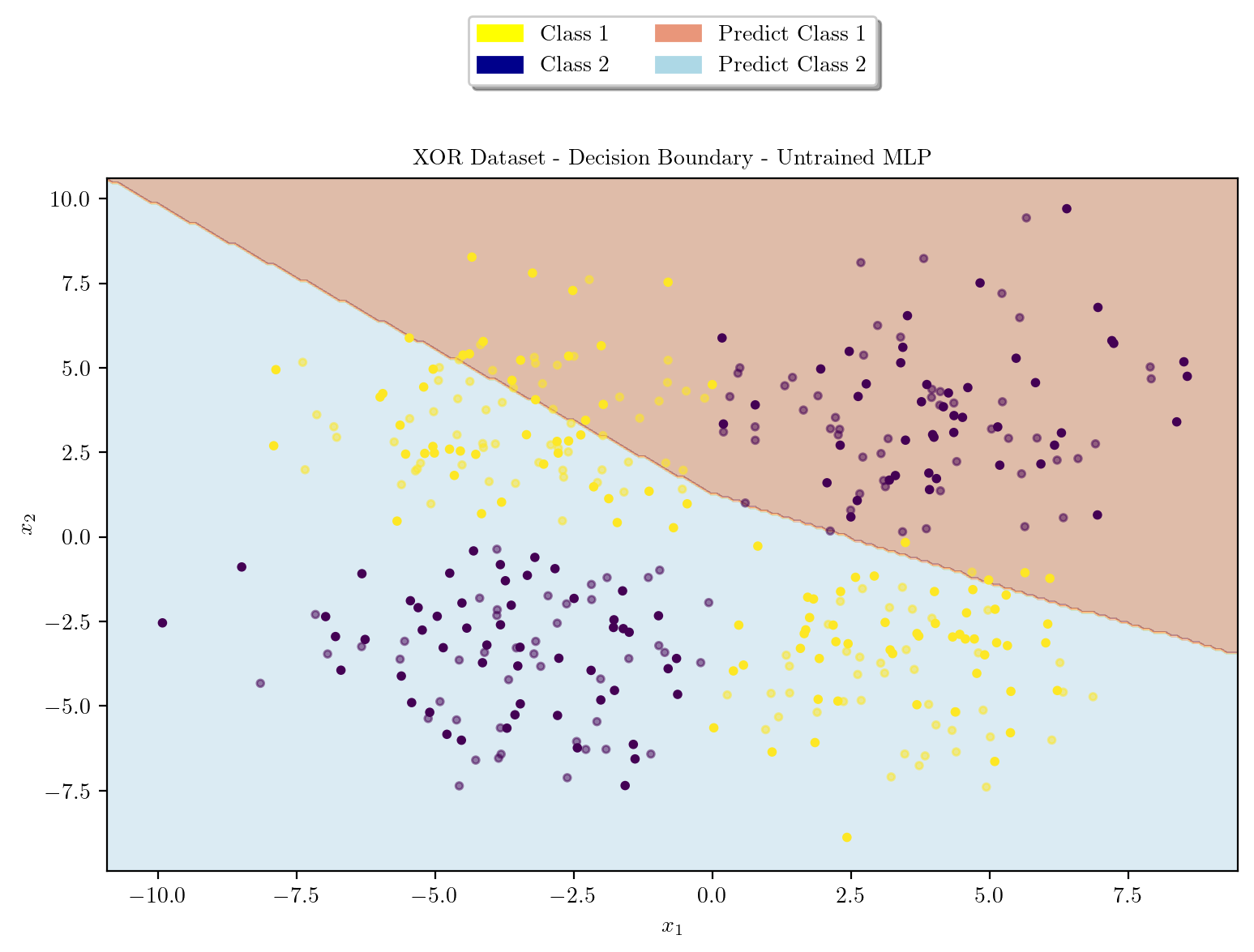

latexify(columns = 2, fig_width = 9)
plot_decision_boundary(X_train, X_test, y_train, y_test, model, r"XOR Dataset - Decision Boundary - MLP with $L_2$ Regularization")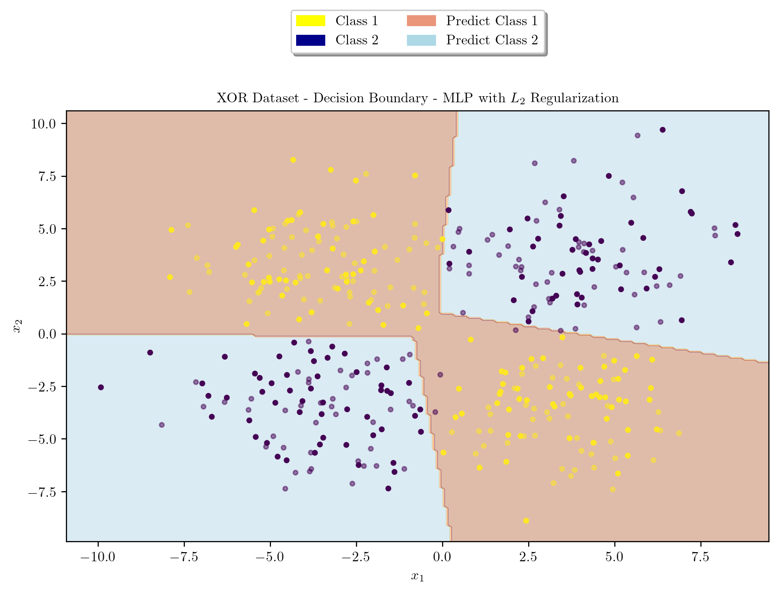

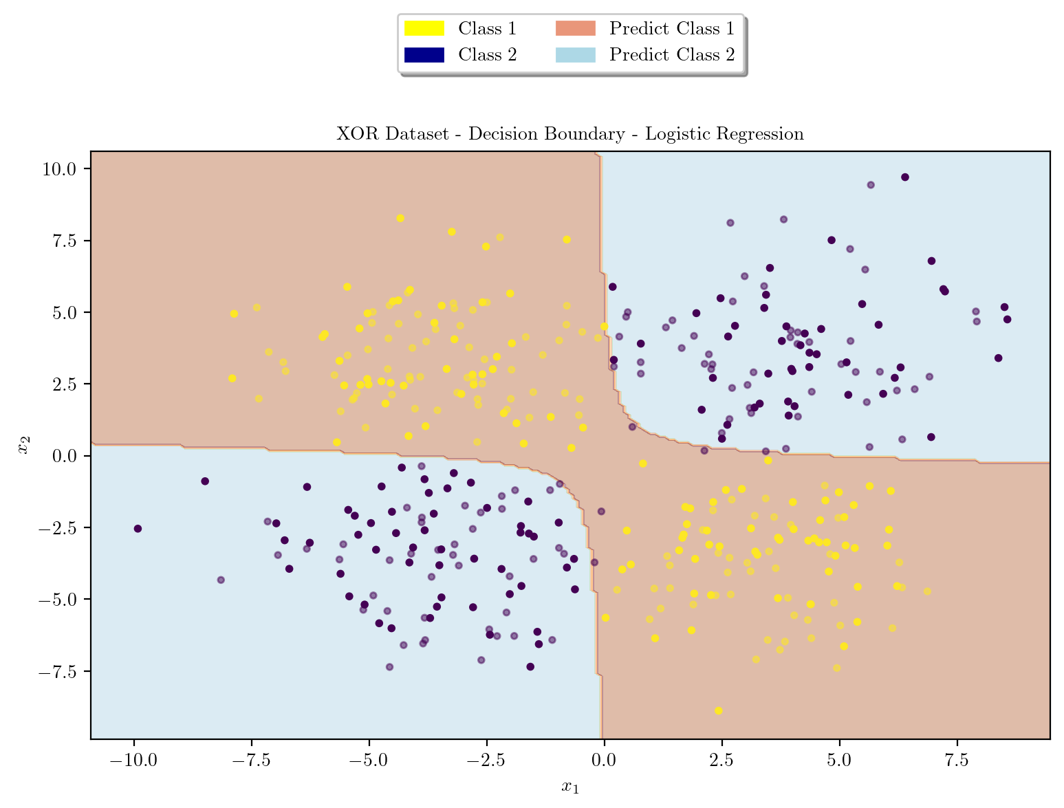
Logistic Regression using Polynomial Features \([x_1^2, x_2^2, x_1x_2]\)

from sklearn.linear_model import LogisticRegression
from sklearn.preprocessing import PolynomialFeatures
from sklearn.metrics import accuracy_score

poly = PolynomialFeatures(degree = 2, include_bias = False)
X_train_poly = poly.fit_transform(X_train)
X_test_poly = poly.transform(X_test)

logreg = LogisticRegression()
logreg.fit(X_train_poly, y_train)

y_train_pred = logreg.predict(X_train_poly)
y_test_pred = logreg.predict(X_test_poly)

train_accuracy = accuracy_score(y_train, y_train_pred)
test_accuracy = accuracy_score(y_test, y_test_pred)

print("Train Accuracy: ", train_accuracy)
print("Test Accuracy: ", test_accuracy)

Train Accuracy:  1.0
Test Accuracy:  0.98

/Users/guntas13/micromamba/lib/python3.9/site-packages/sklearn/utils/validation.py:1229: DataConversionWarning: A column-vector y was passed when a 1d array was expected. Please change the shape of y to (n_samples, ), for example using ravel().
  y = column_or_1d(y, warn=True)

Plotting Decision Surface for Logistic Regression

def plot_decision_boundary(X_train, X_test, y_train, y_test, model, title):
    X = np.concatenate([X_train, X_test], axis = 0)
    y = np.concatenate([y_train, y_test], axis = 0)

    x_min, x_max = X[:, 0].min() - 1, X[:, 0].max() + 1
    y_min, y_max = X[:, 1].min() - 1, X[:, 1].max() + 1

    xx, yy = np.meshgrid(np.arange(x_min, x_max, 0.1), np.arange(y_min, y_max, 0.1))
    poly = PolynomialFeatures(degree = 2, include_bias = False)
    meshgrid_poly = poly.fit_transform(np.c_[xx.ravel(), yy.ravel()])

    Z = model.predict(meshgrid_poly)

    Z = Z.reshape(xx.shape)

    plt.contourf(xx, yy, Z, cmap = plt.cm.Paired, alpha=0.4)

    plt.scatter(X_train[:, 0], X_train[:, 1], c = y_train, cmap = "viridis", s = 10)
    plt.scatter(X_test[:, 0], X_test[:, 1], c = y_test, cmap = "viridis", s = 10, alpha = 0.5)

    yellow_patch = mpatches.Patch(color = "yellow", label = "Class 1")
    blue_patch = mpatches.Patch(color = "darkblue", label = "Class 2")
    pink_patch = mpatches.Patch(color = "darksalmon", label = "Predict Class 1")
    lblue_patch = mpatches.Patch(color = "lightblue", label = "Predict Class 2")
    plt.legend(handles = [yellow_patch, blue_patch, pink_patch, lblue_patch], loc = "upper center", bbox_to_anchor = (0.5, 1.25), ncol = 2, fancybox = True, shadow = True)

    plt.title(title)
    plt.xlabel(r"$x_1$")
    plt.ylabel(r"$x_2$")
    plt.show()

plot_decision_boundary(X_train_poly, X_test_poly, y_train, y_test, logreg, "XOR Dataset - Decision Boundary - Logistic Regression")