import numpy as np
import matplotlib.pyplot as plt
import scipy.stats as stats
import cv2
import urllib.request
from sympy import *IMPORTING MODULES AND LIBRARIES
Question 1
Plot the PMF and CDF of Bernoulli, Geometric, Binomial, and Poission random variables. Choose various values of parameters.
BERNOULLI RANDOM VARIABLE
# PMF OF BERNOULLI
p1, p2 = 0.4, 0.8
rv_bern1, rv_bern2 = stats.bernoulli(p1), stats.bernoulli(p2)
x = np.array([0, 1])
bernoulli1, bernoulli2 = rv_bern1.pmf(x), rv_bern2.pmf(x)
plt.subplots(figsize = (10, 4))
plt.subplot(1, 2, 1)
plt.plot(x, bernoulli1, "ro", ms = 12)
plt.vlines(x, 0, bernoulli1, colors = "r", lw = 5, alpha = 0.5)
plt.grid()
plt.title(f"PMF of Bernoulli with P = {p1}")
plt.legend([f"P = {p1}"])
plt.xlabel("X (Random Variable)")
plt.ylabel("P(X)")
plt.subplot(1, 2, 2)
plt.plot(x, bernoulli2, "bo", ms = 12)
plt.vlines(x, 0, bernoulli2, colors = "b", lw = 5, alpha = 0.5)
plt.grid()
plt.title(f"PMF of Bernoulli with P = {p2}")
plt.legend([f"P = {p2}"])
plt.xlabel("X (Random Variable)")
plt.ylabel("P(X)")
plt.show()
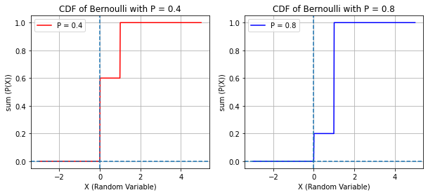
# CDF OF BERNOULLI
x = np.linspace(-3, 5, 500)
bern_cdf1, bern_cdf2 = rv_bern1.cdf(x), rv_bern2.cdf(x)
plt.subplots(figsize = (10, 4))
plt.subplot(1, 2, 1)
plt.plot(x, bern_cdf1, "r-", ms = 12)
plt.axvline(x = 0, linestyle = "--")
plt.axhline(y = 0, linestyle = "--")
plt.legend([f"P = {p1}"])
plt.grid()
plt.title(f"CDF of Bernoulli with P = {p1}")
plt.xlabel("X (Random Variable)")
plt.ylabel("sum (P(X))")
plt.subplot(1, 2, 2)
plt.plot(x, bern_cdf2, "b-", ms = 12)
plt.legend([f"P = {p2}"])
plt.axvline(x = 0, linestyle = "--")
plt.axhline(y = 0, linestyle = "--")
plt.grid()
plt.title(f"CDF of Bernoulli with P = {p2}")
plt.xlabel("X (Random Variable)")
plt.ylabel("sum (P(X))")
plt.show()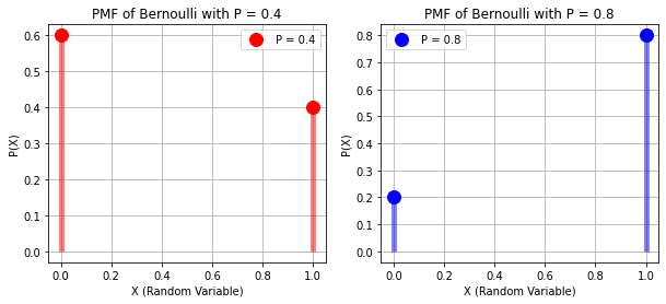
BINOMIAL RANDOM VARIABLE
# PMF OF BINOMIAL
x = np.arange(11)
n, p1, p2 = 10, 0.2, 0.6
rv_bin1, rv_bin2 = stats.binom(n, p1), stats.binom(n, p2)
binomial1 = rv_bin1.pmf(x)
binomial2 = rv_bin2.pmf(x)
plt.subplots(figsize = (10, 4))
plt.subplot(1, 2, 1)
plt.plot(x, binomial1, "go", ms = 10)
plt.vlines(x, 0, binomial1, colors = "g", lw = 5, alpha = 0.5)
plt.legend([f"(N, p) = ({n}, {p1})"])
plt.grid()
plt.title(f"PMF of Binomial with (N, p) = ({n}, {p1})")
plt.xlabel("X (Random Variable)")
plt.ylabel("P(X)")

plt.subplot(1, 2, 2)
plt.plot(x, binomial2, "co", ms = 10)
plt.vlines(x, 0, binomial2, colors = "c", lw = 5, alpha = 0.5)
plt.legend([f"(N, p) = ({n}, {p2})"])
plt.grid()
plt.title(f"PMF of Binomial with (N, p) = ({n}, {p2})")
plt.xlabel("X (Random Variable)")
plt.ylabel("P(X)")
plt.show()

# CDF OF BINOMIAL
x = np.linspace(-3, 12, 500)
bern_cdf1, bern_cdf2 = rv_bin1.cdf(x), rv_bin2.cdf(x)
plt.subplots(figsize = (10, 4))
plt.subplot(1, 2, 1)
plt.plot(x, bern_cdf1, 'g-', ms = 10)
plt.axvline(x = 0, linestyle = "--")
plt.axhline(y = 0, linestyle = "--")
plt.legend([f"(N, p) = ({n}, {p1})"])
plt.title(f"CDF of Bernoulli (N, p) = ({n}, {p1})")
plt.xlabel("X (Random Variable)")
plt.ylabel("sum (P(X))")
plt.grid()

plt.subplot(1, 2, 2)
plt.plot(x, bern_cdf2, 'c-', ms = 10)
plt.legend([f"(N, p) = ({n}, {p2})"])
plt.axvline(x = 0, linestyle = "--")
plt.axhline(y = 0, linestyle = "--")
plt.title(f"CDF of Bernoulli (N, p) = ({n}, {p2})")
plt.xlabel("X (Random Variable)")
plt.ylabel("sum (P(X))")
plt.grid()
plt.show()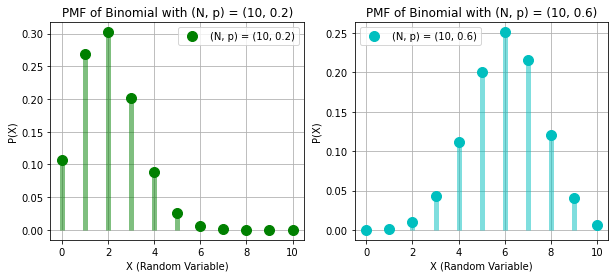

GEOMETRIC RANDOM VARIABLE
# PMF OF GEOMETRIC
x = np.arange(1,14)
p1, p2 = 0.2, 0.6
rv_geom1, rv_geom2 = stats.geom(p1), stats.geom(p2)
geometric1, geometric2 = rv_geom1.pmf(x), rv_geom2.pmf(x)
plt.subplots(figsize = (10, 4))
plt.subplot(1, 2, 1)
plt.plot(x, geometric1, "yo", ms = 10)
plt.vlines(x, 0, geometric1, colors = "y", lw = 5, alpha = 0.5)
plt.legend([f"P = {p1}"])
plt.title(f"PMF of Geometric with P = {p1}")
plt.xlabel("X (Random Variable)")
plt.ylabel("P(X)")
plt.grid()

plt.subplot(1, 2, 2)
plt.plot(x, geometric2, "mo", ms = 10)
plt.vlines(x, 0, geometric2, colors = "m", lw = 5, alpha = 0.5)
plt.legend([f"P = {p2}"])
plt.title(f"PMF of Geometric with P = {p2}")
plt.xlabel("X (Random Variable)")
plt.ylabel("P(X)")
plt.grid()
plt.show()


# CDF OF GEOMETRIC
x = np.linspace(-2, 18, 1000)
geom_cdf1, geom_cdf2 = rv_geom1.cdf(x), rv_geom2.cdf(x)
plt.subplots(figsize = (10, 4))
plt.subplot(1, 2, 1)
plt.plot(x, geom_cdf1, 'y-', ms = 10)
plt.legend([f"P = {p1}"])
plt.axvline(x = 0, linestyle = "--")
plt.axhline(y = 0, linestyle = "--")
plt.title(f"CDF of Geometric with P = {p1}")
plt.xlabel("X (Random Variable)")
plt.ylabel("sum (P(X))")
plt.grid()

plt.subplot(1, 2, 2)
plt.plot(x, geom_cdf2, 'm-', ms = 10)
plt.legend([f"P = {p2}"])
plt.axvline(x = 0, linestyle = "--")
plt.axhline(y = 0, linestyle = "--")
plt.title(f"CDF of Geometric with P = {p2}")
plt.xlabel("X (Random Variable)")
plt.ylabel("sum (P(X))")
plt.grid()
plt.show()
POISSON RANDOM VARIABLE
# PMF OF POISSON
lambd1, lambd2 = 4, 8
x = np.arange(0, 15)
rv_pois1, rv_pois2 = stats.poisson(lambd1), stats.poisson(lambd2)
poisson1, poisson2 = rv_pois1.pmf(x), rv_pois2.pmf(x)
plt.subplots(figsize = (10, 4))
plt.subplot(1, 2, 1)
plt.plot(x, poisson1, "o", color = "orange", ms = 8)
plt.vlines(x, 0, poisson1, colors = "orange", lw = 5, alpha = 0.5)
plt.legend([f"λ = {lambd1}"])
plt.title(f"PMF of Poisson with λ = {lambd1}")
plt.xlabel("X (Random Variable)")
plt.ylabel("P(X)")
plt.grid()

plt.subplot(1, 2, 2)
plt.plot(x, poisson2, "o", color = "cyan", ms = 8)
plt.vlines(x, 0, poisson2, colors = "cyan", lw = 5, alpha = 0.5)
plt.legend([f"λ = {lambd2}"])
plt.title(f"PMF of Poisson λ = {lambd2}")
plt.xlabel("X (Random Variable)")
plt.ylabel("P(X)")
plt.grid()
plt.show()


# CDF OF POISSON
x = np.linspace(-1, 18, 1000)
pois_cdf1, pois_cdf2 = rv_pois1.cdf(x), rv_pois2.cdf(x)
plt.subplots(figsize = (10, 4))
plt.subplot(1, 2, 1)
plt.plot(x, pois_cdf1, '-', color = "orange", ms = 10)
plt.legend([f"λ = {lambd1}"])
plt.axvline(x = 0, linestyle = "--")
plt.axhline(y = 0, linestyle = "--")
plt.title(f"CDF of Poisson with λ = {lambd1}")
plt.xlabel("X (Random Variable)")
plt.ylabel("sum (P(X))")
plt.grid()

plt.subplot(1, 2, 2)
plt.plot(x, pois_cdf2, '-', color = "cyan", ms = 10)
plt.legend([f"λ = {lambd2}"])
plt.axvline(x = 0, linestyle = "--")
plt.axhline(y = 0, linestyle = "--")
plt.title(f"CDF of Poisson λ = {lambd2}")
plt.xlabel("X (Random Variable)")
plt.ylabel("sum (P(X))")
plt.grid()
plt.show()
Question 2
Show the equivalence and the difference between various choices of parameters for Binomial and Poission distributions. Use both PMF and CDF.
# CASE 1
n, p = 50, 0.8
bin_values = np.arange(0, n+1)
bin_probs = stats.binom.pmf(bin_values, n, p)
plt.stem(bin_values, bin_probs, "g")
lambd = n * p
rv2 = stats.poisson(lambd)
x_values = np.arange(0, 100)
f = rv2.pmf(x_values)
plt.plot(x_values, f, color = "magenta")
plt.legend([f"Poisson with λ = N * p", f"Binomial with ({n}, {p})"])
plt.xlim([0, 70])
plt.ylim([0, 0.16])
plt.xlabel("Random Varible (X)")
plt.ylabel("P(X)")
plt.title(f"Both DO NOT MATCH as N ({n}) is SMALL and p ({p}) is LARGE")
plt.grid()
plt.show()
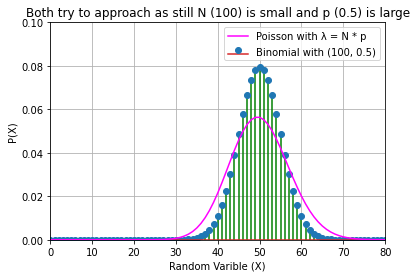
# CASE 2
n, p = 100, 0.5
bin_values = np.arange(0, n+1)
bin_probs = stats.binom.pmf(bin_values, n, p)
plt.stem(bin_values, bin_probs, "g")
lambd = n * p
rv2 = stats.poisson(lambd)
x_values = np.arange(0, 100)
f = rv2.pmf(x_values)
plt.plot(x_values, f, color = "magenta")
plt.legend([f"Poisson with λ = N * p", f"Binomial with ({n}, {p})"])
plt.xlim([0, 80])
plt.ylim([0, 0.1])
plt.xlabel("Random Varible (X)")
plt.ylabel("P(X)")
plt.title(f"Both try to approach as still N ({n}) is small and p ({p}) is large")
plt.grid()
plt.show()
# CASE 3
n, p = 1000, 0.05
bin_values = np.arange(0, n+1)
bin_probs = stats.binom.pmf(bin_values, n, p)
plt.stem(bin_values, bin_probs, "g")
lambd = n * p
rv2 = stats.poisson(lambd)
x_values = np.arange(0, 100)
f = rv2.pmf(x_values)
plt.plot(x_values, f, color = "magenta")
plt.legend([f"Poisson with λ = N * p", f"Binomial with ({n}, {p})"])
plt.xlim([0, 80])
plt.ylim([0, 0.06])
plt.xlabel("Random Varible (X)")
plt.ylabel("P(X)")
plt.title(f"Both MATCH as N ({n}) is LARGE and p ({p}) is SMALL")
plt.grid()
plt.show()
print("HENCE AS N TENDS TO INFINITY AND p TENDS TO 0,\nTHE BINOMIAL RANDOM VARIABLE ACTUALLY BECOMES THE POISSON\nWHOSE λ = N * p")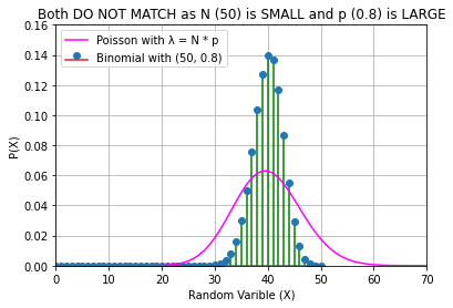
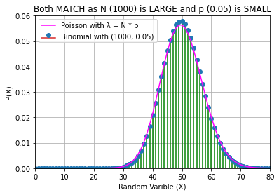
HENCE AS N TENDS TO INFINITY AND p TENDS TO 0,
THE BINOMIAL RANDOM VARIABLE ACTUALLY BECOMES THE POISSON
WHOSE λ = N * p
Question 3
Read an image and add different amounts of Gaussian Noise and display the corrupted images.
COLORED IMAGE
url = urllib.request.urlopen("https://source.unsplash.com/fusZEKsVZL0")
arr = np.asarray(bytearray(url.read()), dtype = np.uint8)
img = cv2.imdecode(arr, -1)
# print(img.shape)
gaussian_noise = np.zeros(img.shape, dtype = np.uint8)
mean, sigma = 100, 100

cv2.randn(gaussian_noise, mean, sigma)
gaussian_noise = (gaussian_noise * 0.5).astype(np.uint8)
gn_img = cv2.add(img, gaussian_noise)

fig = plt.figure(dpi = 300)
fig.add_subplot(1, 3, 1)
plt.imshow(cv2.cvtColor(img, cv2.COLOR_BGR2RGB))
plt.axis("off")
plt.title("Colored Image")

fig.add_subplot(1, 3, 2)
plt.imshow(gaussian_noise, cmap = "gray")
plt.axis("off")
plt.title("Gaussian Noise")

fig.add_subplot(1, 3, 3)
plt.imshow(cv2.cvtColor(gn_img, cv2.COLOR_BGR2RGB))
plt.axis("off")
plt.title("Final Image")
plt.show()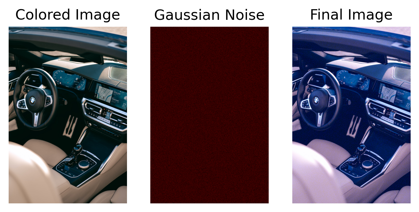
BLACK & WHITE IMAGE
url = urllib.request.urlopen("https://source.unsplash.com/fusZEKsVZL0")
arr = np.asarray(bytearray(url.read()), dtype = np.uint8)
img = cv2.imdecode(arr, 0)
# print(img.shape)
gaussian_noise = np.zeros(img.shape, dtype = np.uint8)
mean, sigma = 100, 100

cv2.randn(gaussian_noise, mean, sigma)
gaussian_noise = (gaussian_noise * 0.5).astype(np.uint8)
gn_img = cv2.add(img, gaussian_noise)

fig = plt.figure(dpi = 300)
fig.add_subplot(1, 3, 1)
plt.imshow(cv2.cvtColor(img, cv2.COLOR_BGR2RGB))
plt.axis("off")
plt.title("B&W Image")

fig.add_subplot(1, 3, 2)
plt.imshow(gaussian_noise, cmap = "gray")
plt.axis("off")
plt.title("Gaussian Noise")

fig.add_subplot(1, 3, 3)
plt.imshow(cv2.cvtColor(gn_img, cv2.COLOR_BGR2RGB))
plt.axis("off")
plt.title("Final Image")
plt.show()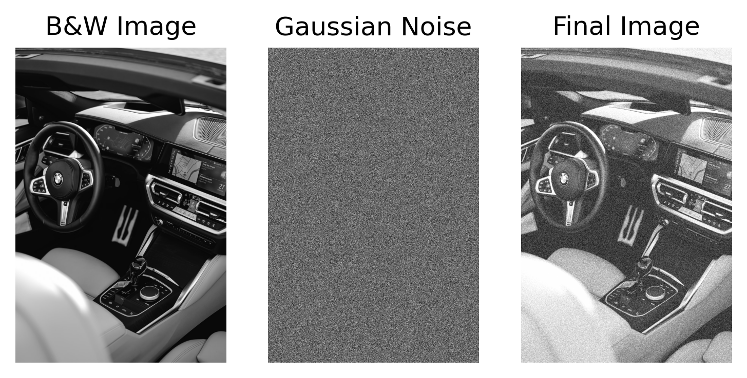
Question 4
Plot the PDF and CDF of the following random variables for different parameter values. - Uniform - Exponential - Rayleigh - Laplacian - Gaussian (Normal) - Chi-square - Erlang - Log-normal - Cauchy - Beta - Weibull
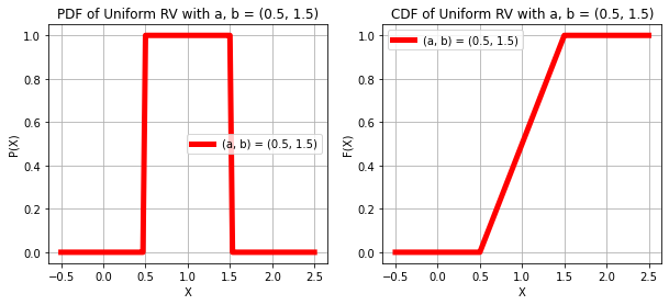
UNIFORM RANDOM VARIABLE
print("X ~ UNIFORM(a, b)")
AB = ((0.1, 0.6), (0.5, 1.5))

x = np.linspace(AB[0][0] - 1 , AB[0][1] + 1, 100), np.linspace(AB[1][0] - 1 , AB[1][1] + 1, 100)

uni_dist1 = stats.uniform(loc = AB[0][0], scale = AB[0][1] - AB[0][0])
uni_dist2 = stats.uniform(loc = AB[1][0], scale = AB[1][1] - AB[1][0])

pdf = uni_dist1.pdf(x[0]), uni_dist2.pdf(x[1])
cdf = uni_dist1.cdf(x[0]), uni_dist2.cdf(x[1])
color = ["green", "red"]
for i in range(2):
  plt.subplots(figsize = (10, 4))
  plt.subplot(1, 2, 1)
  plt.plot(x[i], pdf[i], linewidth = 5, color = color[i])
  plt.title(f"PDF of Uniform RV with a, b = {AB[i]}")
  plt.xlabel("X")
  plt.ylabel("P(X)")
  plt.legend([f"(a, b) = {AB[i]}"])
  plt.grid()

  plt.subplot(1, 2, 2)
  plt.plot(x[i], cdf[i], linewidth = 5, color = color[i])
  plt.title(f"CDF of Uniform RV with a, b = {AB[i]}")
  plt.xlabel("X")
  plt.ylabel("F(X)")
  plt.legend([f"(a, b) = {AB[i]}"])
  plt.grid()
  plt.show()
X ~ UNIFORM(a, b)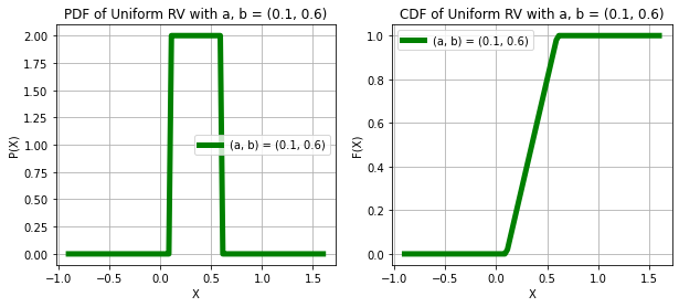
EXPONENTIAL RANDOM VARIABLE
print("X ~ EXPONENTIAL(λ)")
lambd = 0.5, 0.2
x = np.linspace(-0.3, 1.5, 1000)
color = ["blue", "orange"]
for i in range(2):
  f = stats.expon.pdf(x, scale = lambd[i])
  F = stats.expon.cdf(x, scale = lambd[i])
  plt.subplots(figsize = (10, 4))
  plt.subplot(1, 2, 1)
  plt.plot(x, f, color = color[i], linewidth = 4)
  plt.xlabel("X")
  plt.ylabel("P(X)")
  plt.legend([f"λ = {1/lambd[i]}"])
  plt.title(f"PDF of Exponential RV with λ = {1/lambd[i]}")
  plt.grid()
  plt.subplot(1, 2, 2)
  plt.plot(x, F, color = color[i], linewidth = 4)
  plt.xlabel("X")
  plt.ylabel("F(X)")
  plt.legend([f"λ = {1/lambd[i]}"])
  plt.title(f"CDF of Exponential RV with λ = {1/lambd[i]}")
  plt.grid()
  plt.show()
X ~ EXPONENTIAL(λ)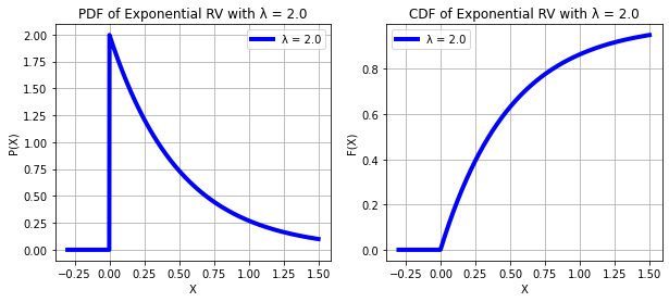
RAYLEIGH RANDOM VARIABLE
print("X ~ RAYLEIGH(s)")
lambd = 1, 5
x = np.linspace(0, 15, 1000)
color = ["pink", "cyan"]
for i in range(2):
  f = stats.rayleigh.pdf(x, scale = lambd[i])
  F = stats.rayleigh.cdf(x, scale = lambd[i])
  plt.subplots(figsize = (10, 4))
  plt.subplot(1, 2, 1)
  plt.plot(x, f, color = color[i], linewidth = 4)
  plt.axvline(x = lambd[i], color = "green", linestyle = "--")
  plt.xlabel("X")
  plt.ylabel("P(X)")
  plt.legend([f"s = {lambd[i]}"])
  plt.title(f"PDF of Rayleigh RV with s = {lambd[i]}")
  plt.grid()
  plt.subplot(1, 2, 2)
  plt.plot(x, F, color = color[i], linewidth = 4)
  plt.xlabel("X")
  plt.ylabel("F(X)")
  plt.legend([f"s = {lambd[i]}"])
  plt.title(f"CDF of Rayleigh RV with s = {lambd[i]}")
  plt.grid()
  plt.show()
print("The mode lies at s")
X ~ RAYLEIGH(s)
The mode lies at s
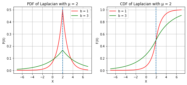
LAPLACIAN RANDOM VARIABLE
print("X ~ LAPLACIAN(µ, b)")
mu = 0, 2
b = 1, 3
x = np.linspace(-7, 7, 1000)

pdf = stats.laplace.pdf(x, mu[0], b[0]), stats.laplace.pdf(x, mu[0], b[1]), stats.laplace.pdf(x, mu[1], b[0]), stats.laplace.pdf(x, mu[1], b[1])
cdf = stats.laplace.cdf(x, mu[0], b[0]), stats.laplace.cdf(x, mu[0], b[1]), stats.laplace.cdf(x, mu[1], b[0]), stats.laplace.cdf(x, mu[1], b[1]),
color = ["red", "green"]
for i in range(0, 3, 2):
  c = 0
  plt.subplots(figsize = (10, 4))
  plt.subplot(1, 2, 1)
  plt.plot(x, pdf[i], color = color[c])
  plt.plot(x, pdf[i + 1], color = color[c + 1])
  plt.axvline(x = mu[i // 2], linestyle = "--")
  plt.legend([f"b = {b[c]}", f"b = {b[c + 1]}"])
  plt.xlabel("X")
  plt.ylabel("P(X)")
  plt.title(f"PDF of Laplacian with µ = {mu[i // 2]}")
  plt.grid()

  plt.subplot(1, 2, 2)
  plt.plot(x, cdf[i], color = color[c])
  plt.plot(x, cdf[i + 1], color = color[c + 1])
  plt.axvline(x = mu[i // 2], linestyle = "--")
  plt.legend([f"b = {b[c]}", f"b = {b[c + 1]}"])
  plt.xlabel('X')
  plt.ylabel('F(X)')
  plt.title(f"CDF of Laplacian with µ = {mu[i // 2]}")
  plt.grid()
  plt.show()
print("Changing the MEAN (µ) shifts the PDF/CDF LEFT or RIGHT\nwhereas, Changing the b, changes the height of the PDF in an inverse manner")
X ~ LAPLACIAN(µ, b)
Changing the MEAN (µ) shifts the PDF/CDF LEFT or RIGHT
whereas, Changing the b, changes the height of the PDF in an inverse manner
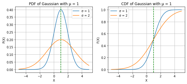
GAUSSIAN(NORMAL) RANDOM VARIABLE
print("X ~ GAUSSIAN(µ, σ^2) or X ~ N(µ, σ^2)")
mu = 0, 1
sigma = 1, 2
x = np.linspace(-5, 5, 1000)

pdf = stats.norm.pdf(x, mu[0], sigma[0]), stats.norm.pdf(x, mu[0], sigma[1]), stats.norm.pdf(x, mu[1], sigma[0]), stats.norm.pdf(x, mu[1], sigma[1])
cdf = stats.norm.cdf(x, mu[0], sigma[0]), stats.norm.cdf(x, mu[0], sigma[1]), stats.norm.cdf(x, mu[1], sigma[0]), stats.norm.cdf(x, mu[1], sigma[1]),

for i in range(0, 3, 2):
  c = 0
  plt.subplots(figsize = (10, 4))
  plt.subplot(1, 2, 1)
  plt.plot(x, pdf[i])
  plt.plot(x, pdf[i + 1])
  plt.axvline(x = mu[i // 2], linestyle = "--", color = "green")
  plt.legend([f"σ = {sigma[c]}", f"σ = {sigma[c + 1]}"])
  plt.xlabel("X")
  plt.ylabel("P(X)")
  plt.title(f"PDF of Gaussian with µ = {mu[i // 2]}")
  plt.grid()

  plt.subplot(1, 2, 2)
  plt.plot(x, cdf[i])
  plt.plot(x, cdf[i + 1])
  plt.axvline(x = mu[i // 2], linestyle = "--", color = "green")
  plt.legend([f"σ = {sigma[c]}", f"σ = {sigma[c + 1]}"])
  plt.xlabel('X')
  plt.ylabel('F(X)')
  plt.title(f"CDF of Gaussian with µ = {mu[i // 2]}")
  plt.grid()
  plt.show()
print("Changing the MEAN (µ) shifts the PDF/CDF LEFT or RIGHT\nwhereas, Changing the Variance(σ^2), STRECHES OR SQUISHES the PDF/CDF")
X ~ GAUSSIAN(µ, σ^2) or X ~ N(µ, σ^2)
Changing the MEAN (µ) shifts the PDF/CDF LEFT or RIGHT
whereas, Changing the Variance(σ^2), STRECHES OR SQUISHES the PDF/CDF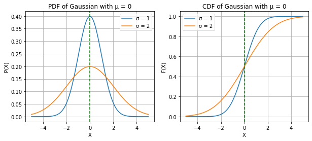
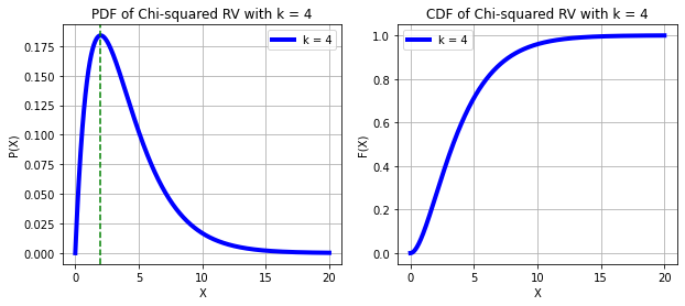
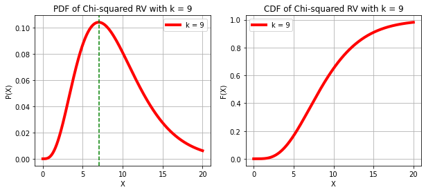
CHI-SQUARE RANDOM VARIABLE
print("X ~ χ^2(k)")
k = 2, 4, 9
x = np.linspace(0, 20, 1000)
color = ["orange", "blue", "red"]
for i in range(3):
  f = stats.chi2.pdf(x, df = k[i])
  F = stats.chi2.cdf(x, df = k[i])
  plt.subplots(figsize = (10, 4))
  plt.subplot(1, 2, 1)
  plt.plot(x, f, color = color[i], linewidth = 4)
  plt.axvline(x = k[i] - 2, color = "green", linestyle = "--")
  plt.xlabel("X")
  plt.ylabel("P(X)")
  plt.legend([f"k = {k[i]}"])
  plt.title(f"PDF of Chi-squared RV with k = {k[i]}")
  plt.grid()
  plt.subplot(1, 2, 2)
  plt.plot(x, F, color = color[i], linewidth = 4)
  plt.xlabel("X")
  plt.ylabel("F(X)")
  plt.legend([f"k = {k[i]}"])
  plt.title(f"CDF of Chi-squared RV with k = {k[i]}")
  plt.grid()
  plt.show()
print("The mode lies at k - 2")
X ~ χ^2(k)
The mode lies at k - 2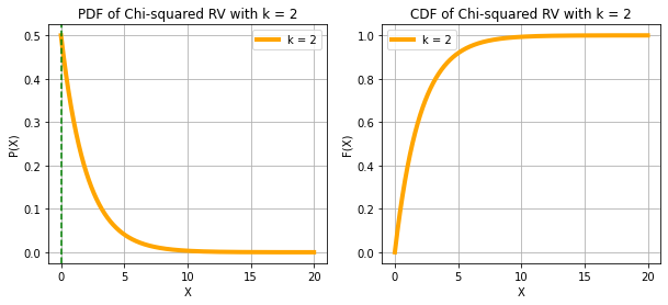
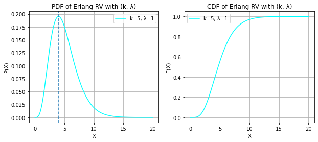
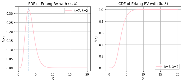
ERLANG RANDOM VARIABLE
print("X ~ ERLANG(k, λ)")
k = 1, 5, 7
lambd = 0.5, 1, 2
x = np.linspace(0, 20, 1000)
color = ["olive", "cyan", "pink"]
for i in range(0, 3):
  pdf = stats.erlang.pdf(x, k[i], scale = 1/lambd[i])
  cdf = stats.erlang.cdf(x, k[i], scale = 1/lambd[i])
  plt.subplots(figsize = (10, 4))
  plt.subplot(1, 2, 1)
  plt.plot(x, pdf, color = color[i])
  plt.axvline(x = (k[i] - 1)/lambd[i], linestyle = "--")
  plt.legend([f"k={k[i]}, λ={lambd[i]}"])
  plt.xlabel("X")
  plt.ylabel("P(X)")
  plt.title(f"PDF of Erlang RV with (k, λ)")
  plt.grid()

  plt.subplot(1, 2, 2)
  plt.plot(x, cdf, color = color[i])
  plt.legend([f"k={k[i]}, λ={lambd[i]}"])
  plt.xlabel('X')
  plt.ylabel('F(X)')
  plt.title(f"CDF of Erlang RV with (k, λ)")
  plt.grid()
  plt.show()
print("The mode now lies at (k - 1)/λ")
X ~ ERLANG(k, λ)
The mode now lies at (k - 1)/λ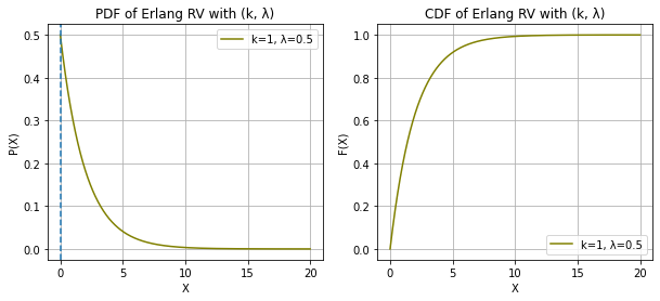
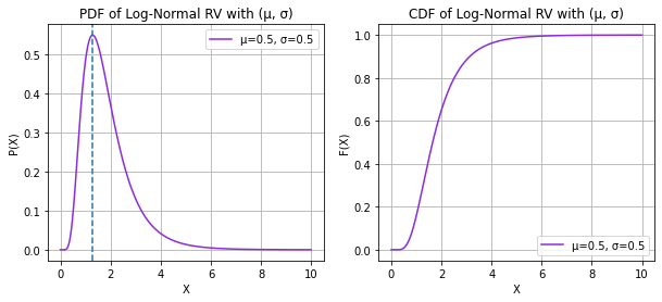
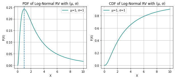
LOG-NORMAL RANDOM VARIABLE
print("X ~ LOGNORMAL(µ, σ^2)\nOR\nLOG(X) ~ GAUSSIAN(µ, σ^2)")
mu = 0, 0.5, 1
sigma = 0.25, 0.5, 1
x = np.linspace(0, 10, 1000)
color = ["crimson", "blueviolet", "teal"]
for i in range(0, 3):
  pdf = stats.lognorm.pdf(x, sigma[i], scale = np.exp(mu[i]))
  cdf = stats.lognorm.cdf(x, sigma[i], scale = np.exp(mu[i]))
  plt.subplots(figsize = (10, 4))
  plt.subplot(1, 2, 1)
  plt.plot(x, pdf, color = color[i])
  plt.axvline(x = np.exp(mu[i] - sigma[i]**2), linestyle = "--")
  plt.legend([f"µ={mu[i]}, σ={sigma[i]}"])
  plt.xlabel("X")
  plt.ylabel("P(X)")
  plt.title(f"PDF of Log-Normal RV with (µ, σ)")
  plt.grid()

  plt.subplot(1, 2, 2)
  plt.plot(x, cdf, color = color[i])
  plt.legend([f"µ={mu[i]}, σ={sigma[i]}"])
  plt.xlabel('X')
  plt.ylabel('F(X)')
  plt.title(f"CDF of Log-Normal RV with (µ, σ)")
  plt.grid()
  plt.show()
print("The mode now lies at exp(µ - σ^2)")
X ~ LOGNORMAL(µ, σ^2)
OR
LOG(X) ~ GAUSSIAN(µ, σ^2)
The mode now lies at exp(µ - σ^2)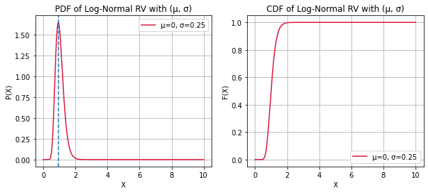
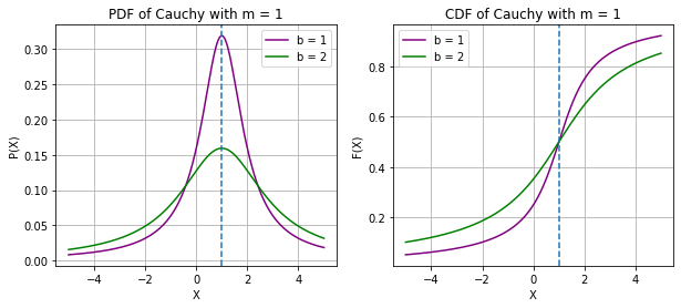
CAUCHY RANDOM VARIABLE
print("X ~ CAUCHY(m, b)")
mu = 0, 1
b = 1, 2
x = np.linspace(-5, 5, 1000)

pdf = stats.cauchy.pdf(x, mu[0], b[0]), stats.cauchy.pdf(x, mu[0], b[1]), stats.cauchy.pdf(x, mu[1], b[0]), stats.cauchy.pdf(x, mu[1], b[1])
cdf = stats.cauchy.cdf(x, mu[0], b[0]), stats.cauchy.cdf(x, mu[0], b[1]), stats.cauchy.cdf(x, mu[1], b[0]), stats.cauchy.cdf(x, mu[1], b[1]),
color = ["purple", "green"]
for i in range(0, 3, 2):
  c = 0
  plt.subplots(figsize = (10, 4))
  plt.subplot(1, 2, 1)
  plt.plot(x, pdf[i], color = color[c])
  plt.plot(x, pdf[i + 1], color = color[c + 1])
  plt.axvline(x = mu[i // 2], linestyle = "--")
  plt.legend([f"b = {b[c]}", f"b = {b[c + 1]}"])
  plt.xlabel("X")
  plt.ylabel("P(X)")
  plt.title(f"PDF of Cauchy with m = {mu[i // 2]}")
  plt.grid()

  plt.subplot(1, 2, 2)
  plt.plot(x, cdf[i], color = color[c])
  plt.plot(x, cdf[i + 1], color = color[c + 1])
  plt.axvline(x = mu[i // 2], linestyle = "--")
  plt.legend([f"b = {b[c]}", f"b = {b[c + 1]}"])
  plt.xlabel('X')
  plt.ylabel('F(X)')
  plt.title(f"CDF of Cauchy with m = {mu[i // 2]}")
  plt.grid()
  plt.show()
print("Changing the m shifts the PDF/CDF LEFT or RIGHT\nwhereas, Changing the b, changes the height of the PDF in an inverse manner")
X ~ CAUCHY(m, b)
Changing the m shifts the PDF/CDF LEFT or RIGHT
whereas, Changing the b, changes the height of the PDF in an inverse manner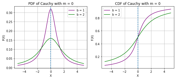
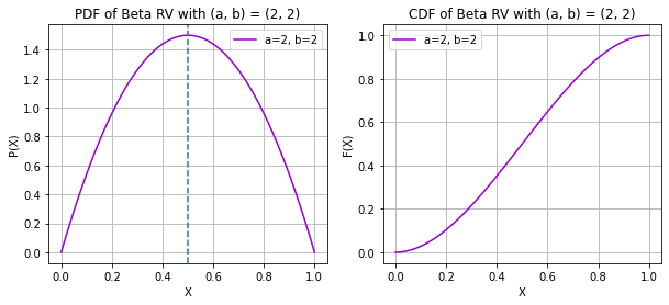
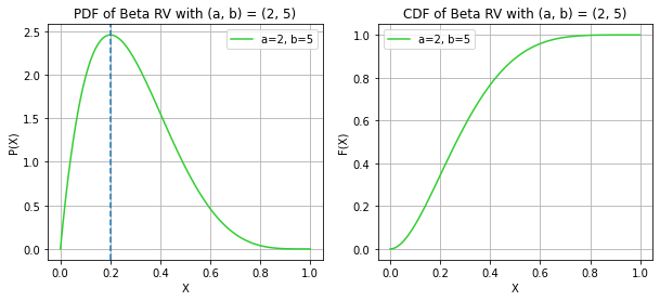
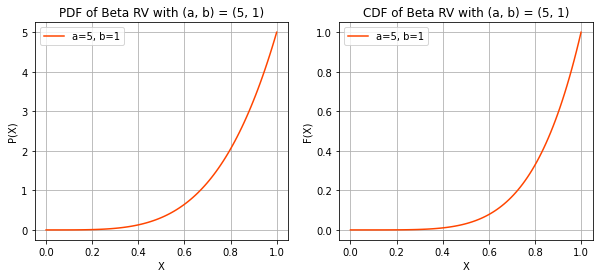
BETA RANDOM VARIABLE
print("X ~ BETA(a, b)")
a = 0.5, 2, 2, 5
b = 0.5, 2, 5, 1
x = np.linspace(0, 1, 100)
color = ["chartreuse", "darkviolet", "limegreen", "orangered"]
for i in range(4):
  pdf = stats.beta.pdf(x, a[i], b[i])
  cdf = stats.beta.cdf(x, a[i], b[i])
  plt.subplots(figsize = (10, 4))
  plt.subplot(1, 2, 1)
  plt.plot(x, pdf, color = color[i])
  if (a[i] > 1 and b[i] > 1):
    plt.axvline(x = (a[i] - 1)/(a[i] + b[i] - 2), linestyle = "--")
  plt.legend([f"a={a[i]}, b={b[i]}"])
  plt.xlabel("X")
  plt.ylabel("P(X)")
  plt.title(f"PDF of Beta RV with (a, b) = ({a[i]}, {b[i]})")
  plt.grid()

  plt.subplot(1, 2, 2)
  plt.plot(x, cdf, color = color[i])
  plt.legend([f"a={a[i]}, b={b[i]}"])
  plt.xlabel('X')
  plt.ylabel('F(X)')
  plt.title(f"CDF of Beta RV with (a, b) = ({a[i]}, {b[i]})")
  plt.grid()
  plt.show()
print("The mode now lies at (a - 1)/(a + b - 2) if a, b > 1 and can vary for other values")
X ~ BETA(a, b)
The mode now lies at (a - 1)/(a + b - 2) if a, b > 1 and can vary for other values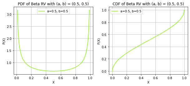
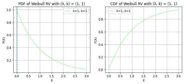
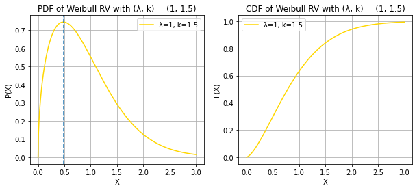
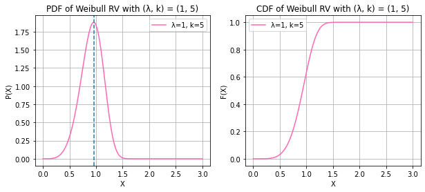
WEIBULL RANDOM VARIABLE
print("X ~ WEIBULL(λ, k)")
k = 0.5, 1, 1.5, 5
lambd = 1, 1, 1, 1
x = np.linspace(0, 3, 500)
color = ["deepskyblue", "palegreen", "gold", "hotpink"]
for i in range(4):
  pdf = stats.weibull_min.pdf(x, k[i], scale = 1/lambd[i])
  cdf = stats.weibull_min.cdf(x, k[i], scale = 1/lambd[i])
  plt.subplots(figsize = (10, 4))
  plt.subplot(1, 2, 1)
  plt.plot(x, pdf, color = color[i])
  if k[i] > 1:
    plt.axvline(x = lambd[i] * ((k[i] - 1)/k[i])**(1 / k[i]), linestyle = "--")
  else:
    plt.axvline(x = 0, linestyle = "--")
  plt.legend([f"λ={lambd[i]}, k={k[i]}"])
  plt.xlabel("X")
  plt.ylabel("P(X)")
  plt.title(f"PDF of Weibull RV with (λ, k) = ({lambd[i]}, {k[i]})")
  plt.grid()

  plt.subplot(1, 2, 2)
  plt.plot(x, cdf, color = color[i])
  plt.legend([f"λ={lambd[i]}, k={k[i]}"])
  plt.xlabel('X')
  plt.ylabel('F(X)')
  plt.title(f"CDF of Weibull RV with (λ, k) = ({lambd[i]}, {k[i]})")
  plt.grid()
  plt.show()
print("The mode now lies at λ * ((k - 1)/k)^(1/k) for k > 1 and at 0 for k =< 1")
X ~ WEIBULL(λ, k)
The mode now lies at λ * ((k - 1)/k)^(1/k) for k > 1 and at 0 for k =< 1/usr/local/lib/python3.9/dist-packages/scipy/stats/_continuous_distns.py:2267: RuntimeWarning: divide by zero encountered in power
return c*pow(x, c-1)*np.exp(-pow(x, c))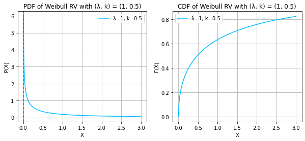
Question 5
Find the Expectation and variance for all the random variables in Question 1 & 4. Further, find and/or plot their characteristic functions.
prob, j, w, mt, lamb, bt, sig, nt, at, st, kt = symbols("p j ω µ λ b σ n a s k")
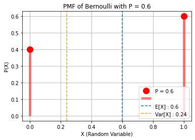
## X ~ BERNOUILLI(p)
p = 0.6
m, v = stats.bernoulli.stats(p, moments = "mv")
expr = 1 - prob + prob*exp(j*w)
print(f"\n1.) X ~ BERNOUILLI(p = {p}):\nE[X]:")
display(prob)
print("Var[X]:")
display(prob * (1 - prob))
print("Characteristic Function φ(ω)=")
display(expr)
print(f"E[X] : {m}\nVar[X] : {v}\n")
x = np.array([0, 1])
bernoulli = stats.bernoulli(p).pmf(x)
plt.plot(x, bernoulli, "ro", ms = 12)
plt.vlines(x, 0, bernoulli, colors = "r", lw = 5, alpha = 0.5)
plt.axvline(x = m, linestyle = "--")
plt.axvline(x = v, linestyle = "--", color = "orange")
plt.legend([f"P = {p}", "", f"E[X] : {m}", f"Var[X] : {v}"])
plt.grid()
plt.title(f"PMF of Bernoulli with P = {p}")
plt.xlabel("X (Random Variable)")
plt.ylabel("P(X)")
plt.show()
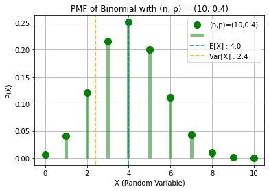
## X ~ BINOMIAL(n, p)
n, p = 10, 0.4
m, v = stats.binom.stats(n, p, moments = "mv")
expr = (1 - prob + prob*exp(j*w))**nt
print(f"\n2.) X ~ BINOMIAL(n = {n}, p = {p}):\nE[X]:")
display(nt * prob)
print("Var[X]:")
display(nt * prob * (1 - prob))
print("Characteristic Function φ(ω) =")
display(expr)
print(f"E[X] : {m}\nVar[X] : {v}\n")
x = np.arange(n + 1)
binomial = stats.binom(n, p).pmf(x)
plt.plot(x, binomial, "go", ms = 10)
plt.vlines(x, 0, binomial, colors = "g", lw = 5, alpha = 0.5)
plt.axvline(x = m, linestyle = "--")
plt.axvline(x = v, linestyle = "--", color = "orange")
plt.legend([f"(n,p)=({n},{p})", "", f"E[X] : {m}", f"Var[X] : {v}"])
plt.grid()
plt.title(f"PMF of Binomial with (n, p) = ({n}, {p})")
plt.xlabel("X (Random Variable)")
plt.ylabel("P(X)")
plt.show()
## X ~ GEOMETRIC(p)
p = 0.2
m, v = stats.geom.stats(p, moments = "mv")
expr = prob * exp(j * w)/(1 - (1 - prob)*exp(j * w))
print(f"\n3.) X ~ GEOMETRIC(p = {p}):\nE[X]:")
display(1/prob)
print("Var[X]:")
display((1 - prob)/prob**2)
print("Characteristic Function φ(ω) =")
display(expr)
print(f"E[X] : {m}\nVar[X] : {v}\n")
x = np.arange(1,v+1)
geometric = stats.geom(p).pmf(x)
plt.plot(x, geometric, "yo", ms = 10)
plt.vlines(x, 0, geometric, colors = "y", lw = 5, alpha = 0.5)
plt.axvline(x = m, linestyle = "--")
plt.axvline(x = v, linestyle = "--", color = "orange")
plt.legend([f"P = {p}", "", f"E[X] : {m}", f"Var[X] : {v}"])
plt.title(f"PMF of Geometric with P = {p}")
plt.xlabel("X (Random Variable)")
plt.ylabel("P(X)")
plt.grid()
plt.show()
## X ~ POISSON(λ)
lambd = 4
m, v = stats.poisson.stats(lambd, moments = "mv")
expr = exp(lamb * (exp(j * w) - 1))
print(f"\n4.) X ~ POISSON(λ = {lambd}):\nE[X]:")
display(lamb)
print("Var[X]:")
display(lamb)
print("Characteristic Function φ(ω) =")
display(expr)
print(f"E[X] : {m}\nVar[X] : {v}\n")
x = np.arange(0, 15)
poisson = stats.poisson(lambd).pmf(x)
plt.plot(x, poisson, "o", color = "orange", ms = 8)
plt.vlines(x, 0, poisson, colors = "orange", lw = 5, alpha = 0.5)
plt.axvline(x = m, linestyle = "--")
plt.axvline(x = v, linestyle = "--", color = "orange")
plt.legend([f"λ = {lambd}", "", f"E[X] : {m}", f"Var[X] : {v}"])
plt.title(f"PMF of Poisson with λ = {lambd}")
plt.xlabel("X (Random Variable)")
plt.ylabel("P(X)")
plt.grid()
plt.show()
## X ~ UNIFORM(a, b)
a, b = 0.5, 1.5
m, v = stats.uniform.stats(loc = a, scale = b - a, moments = "mv")
expr = (exp(bt * j * w) - exp(at * j * w))/(j * w * (bt - at))
print(f"\n5.) X ~ UNIFORM(a = {a}, b = {b}):\nE[X]:")
display((at + bt)/2)
print("Var[X]:")
display((bt - at)**2/12)
print("Characteristic Function φ(ω) = ")
display(expr)
print(f"E[X] : {m}\nVar[X] : {v}\n")
x = np.linspace(a - 1, b + 1, 100)
pdf = stats.uniform(loc = a, scale = b - a).pdf(x)
plt.plot(x, pdf, linewidth = 4, color = "purple")
plt.title(f"PDF of Uniform RV with a, b = {(a, b)}")
plt.xlabel("X")
plt.ylabel("P(X)")
plt.axvline(x = m, linestyle = "--")
plt.axvline(x = v, linestyle = "--", color = "orange")
plt.legend([f"(a,b)=({a},{b})", f"E[X] : {m}", f"Var[X] : {v}"])
plt.grid()
plt.show()
## X ~ EXPONENTIAL(λ)
lambd = 0.5
m, v = stats.expon.stats(scale = lambd, moments = "mv")
expr = lamb/(lamb - j*w)
print(f"\n6.) X ~ EXPONENTIAL(λ = {1/lambd}):\nE[X]:")
display(1/lamb)
print("Var[X]:")
display(1/lamb**2)
print("Characteristic Function φ(ω) =")
display(expr)
print(f"E[X] : {m}\nVar[X] : {v}\n")
x = np.linspace(-0.3, 1.5, 1000)
f = stats.expon.pdf(x, scale = lambd)
plt.plot(x, f, color = "blue", linewidth = 4)
plt.xlabel("X")
plt.ylabel("P(X)")
plt.axvline(x = m, linestyle = "--")
plt.axvline(x = v, linestyle = "--", color = "orange")
plt.legend([f"λ = {1/lambd}", f"E[X] : {m}", f"Var[X] : {v}"])
plt.title(f"PDF of Exponential RV with λ = {1/lambd}")
plt.grid()
plt.show()
## X ~ RAYLEIGH(s)
lambd = 5
m, v = stats.rayleigh.stats(scale = lambd, moments = "mv")
prob, j, w, mt, lamb, bt, sig, nt, at, st, kt = symbols("p j ω µ λ b σ n a s k")
expr = 1 - (st * w * exp(- w**2 * st**2 / 2) * sqrt(pi/2) * (erf(st * w/sqrt(2)) - j))
print(f"\n7.) X ~ RAYLEIGH(s = {lambd}):\nE[X]:")
display(st * sqrt(pi/2))
print("Var[X]:")
display(st**2 * (4 - pi)/2)
print("Characteristic Function φ(ω) =")
display(expr)
print(f"E[X] : {m}\nVar[X] : {v}\n")
x = np.linspace(0, 15, 1000)
f = stats.rayleigh.pdf(x, scale = lambd)
plt.plot(x, f, color = "pink", linewidth = 4)
plt.xlabel("X")
plt.ylabel("P(X)")
plt.axvline(x = m, linestyle = "--")
plt.axvline(x = v, linestyle = "--", color = "orange")
plt.legend([f"s = {1/lambd}", f"E[X] : {m}", f"Var[X] : {v}"])
plt.title(f"PDF of Rayleigh RV with s = {lambd}")
plt.grid()
plt.show()
## X ~ LAPLACIAN(µ, b)
mu, b = 2, 2
m, v = stats.laplace.stats(mu, b, moments = "mv")
expr = exp(j * w * mt)/(1 + bt**2 * w**2)
print(f"\n8.) X ~ LAPLACIAN(µ = {mu}, b = {b}):\nE[X]:")
display(mt)
print("Var[X]:")
display(2 * bt**2)
print("Characteristic Function φ(ω) =")
display(expr)
print(f"E[X] : {m}\nVar[X] : {v}\n")
x = np.linspace(-7, 10, 1000)
pdf = stats.laplace.pdf(x, mu, b)
plt.plot(x, pdf, color = "red", linewidth = 4)
plt.xlabel("X")
plt.ylabel("P(X)")
plt.axvline(x = m, linestyle = "--")
plt.axvline(x = v, linestyle = "--", color = "orange")
plt.legend([f"(µ,b)=({mu},{b})", f"E[X] : {m}", f"Var[X] : {v}"])
plt.title(f"PDF of Laplacian with (µ, b) = ({mu}, {b})")
plt.grid()
plt.show()
## X ~ GAUSSIAN(µ, σ^2)
mu, sigma = 1, 2
m, v = stats.norm.stats(mu, sigma, moments = "mv")
expr = exp(mt * j * w - (sig**2 * w**2)/2)
print(f"\n9.) X ~ GAUSSIAN(µ = {mu}, σ^2 = {sigma**2}):\nE[X]:")
display(mt)
print("Var[X]:")
display(sig**2)
print("Characteristic Function φ(ω) =")
display(expr)
print(f"E[X] : {m}\nVar[X] : {v}\n")
x = np.linspace(-5, 7, 1000)
pdf = stats.norm.pdf(x, mu, sigma)
plt.plot(x, pdf, color = "blueviolet", linewidth = 4)
plt.xlabel("X")
plt.ylabel("P(X)")
plt.axvline(x = m, linestyle = "--")
plt.axvline(x = v, linestyle = "--", color = "orange")
plt.legend([f"(µ,σ^2)=({mu},{sigma**2})", f"E[X] : {m}", f"Var[X] : {v}"])
plt.title(f"PDF of Gaussian with (µ, σ^2) = ({mu}, {sigma**2})")
plt.grid()
plt.show()
## X ~ χ^2(k)
k = 4
m, v = stats.chi2.stats(df = k, moments = "mv")
expr = (1 - 2*j*w)**(-kt/2)
print(f"\n10.) X ~ χ^2(k = {k}):\nE[X]:")
display(kt)
print("Var[X]:")
display(2 * kt)
print("Characteristic Function φ(ω) =")
display(expr)
print(f"E[X] : {m}\nVar[X] : {v}\n")
x = np.linspace(0, 20, 1000)
f = stats.chi2.pdf(x, df = k)
plt.plot(x, f, color = "olive", linewidth = 4)
plt.axvline(x = m, linestyle = "--")
plt.axvline(x = v, linestyle = "--", color = "orange")
plt.xlabel("X")
plt.ylabel("P(X)")
plt.legend([f"k = {k}", f"E[X] : {m}", f"Var[X] : {v}"])
plt.title(f"PDF of Chi-squared RV with k = {k}")
plt.grid()
plt.show()
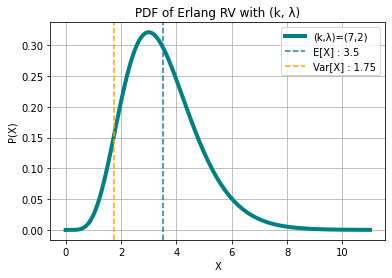
## X ~ ERLANG(k, λ)
k, lambd = 7, 2
m, v = stats.erlang.stats(k, scale = 1/lambd, moments = "mv")
expr = (1 - (j * w)/kt)**(-kt)
print(f"\n11.) X ~ ERLANG(k = {k}, λ = {lambd}):\nE[X]:")
display(kt/lamb)
print("Var[X]:")
display(kt/lamb**2)
print("Characteristic Function φ(ω) =")
display(expr)
print(f"E[X] : {m}\nVar[X] : {v}\n")
x = np.linspace(0, 11, 1000)
pdf = stats.erlang.pdf(x, k, scale = 1/lambd)
plt.plot(x, pdf, color = "teal", linewidth = 4)
plt.axvline(x = m, linestyle = "--")
plt.axvline(x = v, linestyle = "--", color = "orange")
plt.legend([f"(k,λ)=({k},{lambd})", f"E[X] : {m}", f"Var[X] : {v}"])
plt.xlabel("X")
plt.ylabel("P(X)")
plt.title(f"PDF of Erlang RV with (k, λ)")
plt.grid()
plt.show()
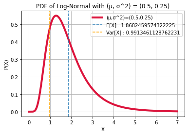
## X ~ LOGNORMAL(µ, σ^2)
mu, sigma = 0.5, 0.5
m, v = stats.lognorm.stats(sigma, scale = np.exp(mu), moments = "mv")
expr = Sum((j * w)**nt/(factorial(nt)) * exp(mt * nt + nt**2 * sig**2/2), (nt, 0, oo))
print(f"\n12.) X ~ LOGNORMAL(µ = {mu}, σ^2 = {sigma**2})):\nE[X]:")
display(exp(mt + sig**2/2))
print("Var[X]:")
display((exp(sig**2) - 1)*exp(2*mt + sig**2))
print("Characteristic Function φ(ω) =")
display(expr)
print(f"E[X] : {m}\nVar[X] : {v}\n")
x = np.linspace(0, 7, 1000)
pdf = stats.lognorm.pdf(x, sigma, scale = np.exp(mu))
plt.plot(x, pdf, color = "crimson", linewidth = 4)
plt.xlabel("X")
plt.ylabel("P(X)")
plt.axvline(x = m, linestyle = "--")
plt.axvline(x = v, linestyle = "--", color = "orange")
plt.legend([f"(µ,σ^2)=({mu},{sigma**2})", f"E[X] : {m}", f"Var[X] : {v}"])
plt.title(f"PDF of Log-Normal with (µ, σ^2) = ({mu}, {sigma**2})")
plt.grid()
plt.show()
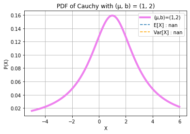
## X ~ CAUCHY(m, b)
mu, b = 1, 2
m, v = stats.cauchy.stats(mu, b, moments = "mv")
print(f"\n13.) X ~ CAUCHY(m = {mu}, b = {b}):\nE[X] = undefined\nVar[X] = undefined\nCharacteristic Function φ(ω) =\nundefined\nE[X] : {m}\nVar[X] : {v}\n")
x = np.linspace(-5, 6, 1000)
pdf = stats.cauchy.pdf(x, mu, b)
plt.plot(x, pdf, color = "violet", linewidth = 4)
plt.xlabel("X")
plt.ylabel("P(X)")
plt.axvline(x = m, linestyle = "--")
plt.axvline(x = v, linestyle = "--", color = "orange")
plt.legend([f"(µ,b)=({mu},{b})", f"E[X] : {m}", f"Var[X] : {v}"])
plt.title(f"PDF of Cauchy with (µ, b) = ({mu}, {b})")
plt.grid()
plt.show()
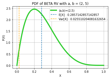
## X ~ BETA(a, b)
a, b = 2, 5
m, v = stats.beta.stats(a, b, moments = "mv")
print(f"\n14.) X ~ BETA(a = {a}, b = {b}):\nE[X]:")
display(at/(at + bt))
print("Var[X]:")
display((at * bt)/((at + bt)**2 * (at + bt + 1)))
print(f"Characteristic Function φ(ω) =\nHIGHLY COMPLEX, requires confluent hypergeometric functions to display in closed form\nE[X] : {m}\nVar[X] : {v}\n")
x = np.linspace(0, 1, 100)
pdf = stats.beta.pdf(x, a, b)
plt.plot(x, pdf, linewidth = 4, color = "limegreen")
plt.title(f"PDF of BETA RV with a, b = {(a, b)}")
plt.xlabel("X")
plt.ylabel("P(X)")
plt.axvline(x = m, linestyle = "--")
plt.axvline(x = v, linestyle = "--", color = "orange")
plt.legend([f"(a,b)=({a},{b})", f"E[X] : {m}", f"Var[X] : {v}"])
plt.grid()
plt.show()
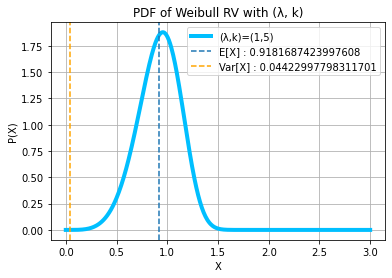
## X ~ WEIBULL(λ, k)
k, lambd = 5, 1
m, v = stats.weibull_min.stats(k, scale = 1/lambd, moments = "mv")
expr = Sum(((j*w)**nt/(factorial(nt)) * lamb**nt * gamma(1 + nt/kt)), (nt, 0, oo))
print(f"\n15.) X ~ WEIBULL(λ = {lambd}, k = {k}):\nE[X]:")
display(lamb * gamma(1 + 1/kt))
print("Var[X]:")
display(lamb**2 * (gamma(1 + 2/kt) - (gamma(1 + 1/kt))**2))
print("Characteristic Function φ(ω) =")
display(expr)
print(f"E[X] : {m}\nVar[X] : {v}\n")
x = np.linspace(0, 3, 500)
pdf = stats.weibull_min.pdf(x, k, scale = 1/lambd)
plt.plot(x, pdf, color = "deepskyblue", linewidth = 4)
plt.axvline(x = m, linestyle = "--")
plt.axvline(x = v, linestyle = "--", color = "orange")
plt.legend([f"(λ,k)=({lambd},{k})", f"E[X] : {m}", f"Var[X] : {v}"])
plt.xlabel("X")
plt.ylabel("P(X)")
plt.title(f"PDF of Weibull RV with (λ, k)")
plt.grid()
plt.show()
1.) X ~ BERNOUILLI(p = 0.6):
E[X]:
Var[X]:
Characteristic Function φ(ω)=
E[X] : 0.6
Var[X] : 0.24


2.) X ~ BINOMIAL(n = 10, p = 0.4):
E[X]:
Var[X]:
Characteristic Function φ(ω) =
E[X] : 4.0
Var[X] : 2.4


3.) X ~ GEOMETRIC(p = 0.2):
E[X]:
Var[X]:
Characteristic Function φ(ω) =
E[X] : 5.0
Var[X] : 20.0


4.) X ~ POISSON(λ = 4):
E[X]:
Var[X]:
Characteristic Function φ(ω) =
E[X] : 4.0
Var[X] : 4.0


5.) X ~ UNIFORM(a = 0.5, b = 1.5):
E[X]:
Var[X]:
Characteristic Function φ(ω) =
E[X] : 1.0
Var[X] : 0.08333333333333333


6.) X ~ EXPONENTIAL(λ = 2.0):
E[X]:
Var[X]:
Characteristic Function φ(ω) =
E[X] : 0.5
Var[X] : 0.25


7.) X ~ RAYLEIGH(s = 5):
E[X]:
Var[X]:
Characteristic Function φ(ω) =
E[X] : 6.2665706865775
Var[X] : 10.730091830127586


8.) X ~ LAPLACIAN(µ = 2, b = 2):
E[X]:
Var[X]:
Characteristic Function φ(ω) =
E[X] : 2.0
Var[X] : 8.0


9.) X ~ GAUSSIAN(µ = 1, σ^2 = 4):
E[X]:
Var[X]:
Characteristic Function φ(ω) =
E[X] : 1.0
Var[X] : 4.0


10.) X ~ χ^2(k = 4):
E[X]:
Var[X]:
Characteristic Function φ(ω) =
E[X] : 4.0
Var[X] : 8.0


11.) X ~ ERLANG(k = 7, λ = 2):
E[X]:
Var[X]:
Characteristic Function φ(ω) =
E[X] : 3.5
Var[X] : 1.75


12.) X ~ LOGNORMAL(µ = 0.5, σ^2 = 0.25)):
E[X]:
Var[X]:
Characteristic Function φ(ω) =
E[X] : 1.8682459574322225
Var[X] : 0.9913461128762231


13.) X ~ CAUCHY(m = 1, b = 2):
E[X] = undefined
Var[X] = undefined
Characteristic Function φ(ω) =
undefined
E[X] : nan
Var[X] : nan


14.) X ~ BETA(a = 2, b = 5):
E[X]:
Var[X]:
Characteristic Function φ(ω) =
HIGHLY COMPLEX, requires confluent hypergeometric functions to display in closed form
E[X] : 0.2857142857142857
Var[X] : 0.025510204081632654


15.) X ~ WEIBULL(λ = 1, k = 5):
E[X]:
Var[X]:
Characteristic Function φ(ω) =
E[X] : 0.9181687423997608
Var[X] : 0.04422997798311701
\(\displaystyle p\)
\(\displaystyle p \left(1 - p\right)\)
\(\displaystyle p e^{j ω} - p + 1\)
\(\displaystyle n p\)
\(\displaystyle n p \left(1 - p\right)\)
\(\displaystyle \left(p e^{j ω} - p + 1\right)^{n}\)
\(\displaystyle \frac{1}{p}\)
\(\displaystyle \frac{1 - p}{p^{2}}\)
\(\displaystyle \frac{p e^{j ω}}{- \left(1 - p\right) e^{j ω} + 1}\)
\(\displaystyle λ\)
\(\displaystyle λ\)
\(\displaystyle e^{λ \left(e^{j ω} - 1\right)}\)
\(\displaystyle \frac{a}{2} + \frac{b}{2}\)
\(\displaystyle \frac{\left(- a + b\right)^{2}}{12}\)
\(\displaystyle \frac{- e^{a j ω} + e^{b j ω}}{j ω \left(- a + b\right)}\)
\(\displaystyle \frac{1}{λ}\)
\(\displaystyle \frac{1}{λ^{2}}\)
\(\displaystyle \frac{λ}{- j ω + λ}\)
\(\displaystyle \frac{\sqrt{2} \sqrt{\pi} s}{2}\)
\(\displaystyle \frac{s^{2} \left(4 - \pi\right)}{2}\)
\(\displaystyle - \frac{\sqrt{2} \sqrt{\pi} s ω \left(- j + \operatorname{erf}{\left(\frac{\sqrt{2} s ω}{2} \right)}\right) e^{- \frac{s^{2} ω^{2}}{2}}}{2} + 1\)
\(\displaystyle µ\)
\(\displaystyle 2 b^{2}\)
\(\displaystyle \frac{e^{j µ ω}}{b^{2} ω^{2} + 1}\)
\(\displaystyle µ\)
\(\displaystyle σ^{2}\)
\(\displaystyle e^{j µ ω - \frac{σ^{2} ω^{2}}{2}}\)
\(\displaystyle k\)
\(\displaystyle 2 k\)
\(\displaystyle \left(- 2 j ω + 1\right)^{- \frac{k}{2}}\)
\(\displaystyle \frac{k}{λ}\)
\(\displaystyle \frac{k}{λ^{2}}\)
\(\displaystyle \left(- \frac{j ω}{k} + 1\right)^{- k}\)
\(\displaystyle e^{µ + \frac{σ^{2}}{2}}\)
\(\displaystyle \left(e^{σ^{2}} - 1\right) e^{2 µ + σ^{2}}\)
\(\displaystyle \sum_{n=0}^{\infty} \frac{\left(j ω\right)^{n} e^{\frac{n^{2} σ^{2}}{2} + n µ}}{n!}\)
\(\displaystyle \frac{a}{a + b}\)
\(\displaystyle \frac{a b}{\left(a + b\right)^{2} \left(a + b + 1\right)}\)
\(\displaystyle λ \Gamma\left(1 + \frac{1}{k}\right)\)
\(\displaystyle λ^{2} \left(- \Gamma^{2}\left(1 + \frac{1}{k}\right) + \Gamma\left(1 + \frac{2}{k}\right)\right)\)
\(\displaystyle \sum_{n=0}^{\infty} \frac{λ^{n} \left(j ω\right)^{n} \Gamma\left(1 + \frac{n}{k}\right)}{n!}\)