Denoising Diffusion Probabilistic Models
As seen in the case of Variational Autoencoders, it all boils down to learning the probability distributions - \(p(\textbf{z} | \textbf{x})\) the posterior abstraction of obtaining a hidden representation \(\textbf{z}\) given some input image \(\textbf{x}\) and the likelihood \(p(\textbf{x} | \textbf{z})\) of generating the image samples given some hidden representation \(\textbf{z}\).
Now the most crucial task in all these generative models is trying to understand to relate the objective that we are trying to acheive and what the model actually learns. We’ll see the same confusing conclusion being established by the end of this blog and then we’ll realise how beautifully all the mathematics and the tasks laid out make sense.
Throwback to Variational Autoencoders
Like in the case of VAEs[1], we started off by approximating the actual \(P(\textbf{z} | \textbf{x})\) through our probabilistic Encoder \(Q_{\phi}(\textbf{z} | \textbf{x})\) and minimising the KL divergence between these two. But in order to establish the knowledge of the actual \(P(\textbf{z} | \textbf{x})\), we went into maximising the log-likelihood of data samples \(\textbf{x}\) and eventually made the encoder learn this distribution \(Q_{\phi}(\textbf{z} | \textbf{x})\) to be as close to the standard normal \(\mathcal{N}(\textbf{0}, \mathbb{I})\) as possible. Hence now drawing any \(\textbf{z} \sim \mathcal{N}(\textbf{0}, \mathbb{I})\) we are sure of it being close to the \(\textbf{z}\)’s seen during training, allowing us to discard off the encoder entirely at inference. The way we setup the objective of making the actual and approximated distribution close to each other will stay same for Diffusion Models too and this would allow us to uncover more truth about the actual distribution itself.
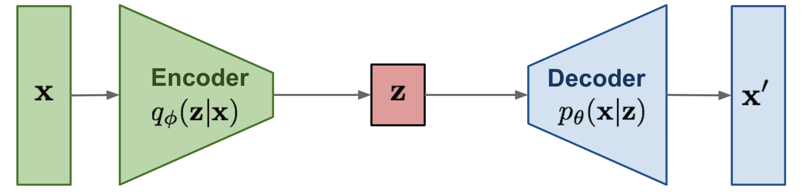
Graphical Model of a Variation Autoencoder.
Adapted from [2].
What are Diffusion Models?
For Diffusion Models instead of one latent variable \(\textbf{z}\), we have \(T\) latent variables of the form \(\textbf{x}_1, \textbf{x}_2, \cdots , \textbf{x}_T\) of same dimension as the input image \(\textbf{x}_0\), and the most interesting point is that the forward noising process is a deterministic Markov Chain, wherein Gaussian noise is added in gradual \(T\) steps, defined as:
\[ \boxed{q(\textbf{x}_t | \textbf{x}_{t - 1}) = \mathcal{N}(\textbf{x}_{t}; \sqrt{1 - \beta_{t}} \textbf{x}_{t - 1}, \beta_{t} \mathbb{I})} \]
Here the variances are controlled by a scheduler \(\left \{ \beta_t \in (0, 1) \right \}_{t = 1}^T\), which means for each noisy sample \(\textbf{x}_t\) is sampled from a Gaussian with \(\boldsymbol{\mu}_q = \sqrt{1 - \beta_{t}} \textbf{x}_{t - 1}\) and covariance matrix \(\mathbf{\Sigma}_q = \beta_{t} \mathbb{I}\). The idea is then to learn the reverse denoising diffusion distribution \(q(\textbf{x}_{t - 1} | \textbf{x}_t)\), which is also a Markov Chain with learned Gaussian transitions[3] starting at \(p(\textbf{x}_T) \sim \mathcal{N}(\textbf{x}_T; \textbf{0}, \mathbb{I})\). Therefore it then becomes really important to understand the entire joint distribution \(p(\textbf{x}_1, \textbf{x}_2, \cdots, \textbf{x}_T)\) denoted in shorthand as \(p(\textbf{x}_{0:T})\)
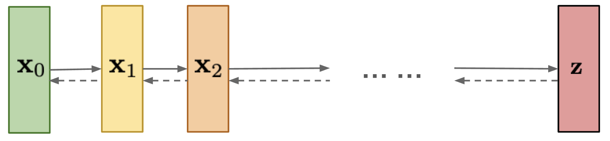
Graphical Model of a Diffusion Process.
Adapted from [2].
Prerequisites
Joint & Conditional Distribution of \(N\) RVs and Bayes’ Rule
A joint distribution over \(N\) random variables assigns probabilities to all the events involving these \(N\) random variables1, denoted as
\[ P(X_1, X_2, X_3, \cdots, X_N) \]
Now starting off with just two RVs, the conditional probabilities \(P(X_1 | X_2)\) and \(P(X_2 | X_1)\) can be calculated from the joint distribution as:
\[ \begin{align} P(X_1 | X_2) = \frac{P(X_1, X_2)}{P(X_2)} && P(X_2 | X_1) = \frac{P(X_1, X_2)}{P(X_1)} \end{align} \]
Conveniently this allows us to write \(P(X_1, X_2) = P(X_2 | X_1) P(X_1)\). And similarly for \(N\) random variables
\[ \begin{align} P(X_1, X_2, X_3, \cdots, X_N) &= P(X_2, X_3, \cdots, X_N | X_1) \cdot P(X_1) \\ &= P(X_3, \cdots, X_N | X_1, X_2) \cdot P(X_2 | X_1) \cdot P(X_1) \\ &= P(X_4, \cdots, X_N | X_1, X_2, X_3) \cdot P(X_3 | X_2, X_1) \cdot P(X_2 | X_1) \cdot P(X_1) \end{align} \]
Expanding by chain rule we get \[ \boxed{P(X_1, X_2, X_3, \cdots, X_N) = P(X_1) \cdot \prod_{i = 2}^{N} P(X_i | X_1^{i - 1})} \]
where \(X_1^{i - 1} = X_1, X_2, X_3, \cdots, X_{i - 1}\) and then using the joint-conditional-marginal formula, we get the Bayes’ Rule as
\[ P(X_2 | X_1) = \frac{P(X_1 | X_2) \cdot P(X_2)}{P(X_1)} \]
Markov-Diffusion Process and Reparametrization
The special property of a Markov Process is that the future state is dependent only on previous state, which means
\[ P(\textbf{x}_t | \textbf{x}_{t - 1}, \cdots, \textbf{x}_0) = P(\textbf{x}_t | \textbf{x}_{t - 1}) \]
the utility of this is that using the chain rule of joint probability, we may simply write for all our diffusion process forward steps \(q(\textbf{x}_{1 : T} | \textbf{x}_0)\) as
\[ \begin{align} q(\textbf{x}_{1 : T} | \textbf{x}_0) = \prod_{t = 1}^{T} q(\textbf{x}_t | \textbf{x}_{t - 1}) && q(\textbf{x}_t | \textbf{x}_{t - 1}) = \mathcal{N}(\textbf{x}_{t}; \sqrt{1 - \beta_{t}} \textbf{x}_{t - 1}, \beta_{t} \mathbb{I}) \end{align} \]
Diffusion is the process of converting samples from a complex distribution (the data here) \(\textbf{x}_0 \sim q(\textbf{x}_0)\) to samples of a simple distribution (isotropic Gaussian noise) \(\textbf{x}_T \sim \mathcal{N}(\textbf{0}, \mathbb{I})\). One can also observe that there is a \(\color{purple}{\text{deterministic}}\) and a \(\color{blue}{\text{stochastic}}\) component even in our case. Since any RV can be reparametrized as \(Z = \sigma X + \mu\), hence we denote the \(\textbf{x}_t\) being drawn from \(q(\textbf{x}_t | \textbf{x}_{t - 1})\) as
\[ \boxed{\textbf{x}_t = \color{purple}{\sqrt{1 - \beta_t} \textbf{x}_{t - 1}} + \color{blue}{\sqrt{\beta_t} \boldsymbol{\epsilon}_{t - 1}}} \]
where \(\boldsymbol{\epsilon}_{t - 1}, \boldsymbol{\epsilon}_{t - 2}, \cdots \sim \mathcal{N}(\textbf{0}, \mathbb{I})\)
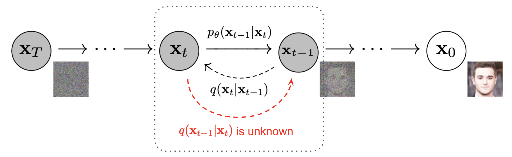
Forward and Reverse Diffusion Processes.
Adapted from [3].
Understanding the Forward Markov Process
One might wonder why does following the above said markov chain of gaussians lead to \(\textbf{x}_T \sim \mathcal{N}(\textbf{0}, \mathbb{I})\). To understand this let’s take arbitrary constants for the above
\[ \textbf{x}_t = \sqrt{\alpha} \textbf{x}_{t - 1} + \sqrt{\beta} \boldsymbol{\epsilon}_{t - 1} \]
Since we know that \(\textbf{x}_T \sim \mathcal{N}(\textbf{0}, \mathbb{I})\) so let’s open up the formula from this end
\[ \begin{align} \textbf{x}_T &= \sqrt{\alpha} \textbf{x}_{T - 1} + \sqrt{\beta} \mathcal{N}(\textbf{0}, \mathbb{I}) \\ &= \sqrt{\alpha} (\sqrt{\alpha} \textbf{x}_{T - 2} + \sqrt{\beta} \mathcal{N}(\textbf{0}, \mathbb{I})) + \sqrt{\beta} \mathcal{N}(\textbf{0}, \mathbb{I}) \\ &= (\sqrt{\alpha})^2 \textbf{x}_{T - 2} + \sqrt{\alpha} \sqrt{\beta} \mathcal{N}(\textbf{0}, \mathbb{I}) + \sqrt{\beta} \mathcal{N}(\textbf{0}, \mathbb{I}) \\ \cdots \\ &= (\sqrt{\alpha})^T \textbf{x}_0 + \sqrt{\beta} ((\sqrt{\alpha})^{T - 1} \mathcal{N}(\textbf{0}, \mathbb{I}) + (\sqrt{\alpha})^{T - 2} \mathcal{N}(\textbf{0}, \mathbb{I}) + \cdots + \mathcal{N}(\textbf{0}, \mathbb{I})) \end{align} \]
We can combine the independent Gaussians into one Gaussian2 as they have variances as \((\beta \alpha^{T - 1}, \beta \alpha^{T - 2}, \cdots, \beta \alpha, \beta)\) with \(\sigma^2 = \beta \frac{1 - \alpha^T}{1 - \alpha}\). Notice that as \(T \to \infty, (\sqrt{\alpha})^T \to 0\) and \(\textbf{x}_T \to \mathcal{N}(\textbf{0}, \mathbb{I})\) only when \(\alpha = 1 - \beta\).
Do we traverse for all \(T\) steps?
Certainly Not! Here’s how the Markov Process allows us to reach any \(\textbf{x}_t\) from the image \(\textbf{x}_0\). Let \(\alpha_t = 1 - \beta_t\)
\[ \begin{align} \textbf{x}_t &= \sqrt{\alpha_t} \textbf{x}_{t - 1} + \sqrt{1 - \alpha_t} \mathcal{N}(\textbf{0}, \mathbb{I}) \\ &= \sqrt{\alpha_t} (\sqrt{\alpha_{t - 1}} \textbf{x}_{t - 2} + \sqrt{1 - \alpha_{t - 1}} \mathcal{N}(\textbf{0}, \mathbb{I})) + \sqrt{1 - \alpha_t} \mathcal{N}(\textbf{0}, \mathbb{I}) \\ &= (\sqrt{\alpha_t \alpha_{t - 1}}) \textbf{x}_{t - 2} + (\sqrt{\alpha_t} \sqrt{1 - \alpha_{t - 1}}) \mathcal{N}(\textbf{0}, \mathbb{I}) + (\sqrt{1 - \alpha_t}) \mathcal{N}(\textbf{0}, \mathbb{I}) \end{align} \]
Combine the independent Gaussians with \(\sigma^2 = \alpha_t (1 - \alpha_{t - 1}) + (1 - \alpha_t) = 1 - \alpha_t \alpha_{t - 1}\), hence
\[ \begin{align} \textbf{x}_t &= (\sqrt{\alpha_t \alpha_{t - 1}}) \textbf{x}_{t - 2} + (\sqrt{1 - \alpha_t \alpha_{t - 1}})\mathcal{N}(\textbf{0}, \mathbb{I}) \\ \cdots \\ &= (\sqrt{\alpha_t \alpha_{t - 1} \cdots \alpha_2 \alpha_1}) \textbf{x}_0 + (\sqrt{1 - \alpha_t \alpha_{t - 1} \cdots \alpha_2 \alpha_1}) \mathcal{N}(\textbf{0}, \mathbb{I}) \end{align} \]
With \(\bar{\alpha_t} = \prod_{i = 1}^{t} \alpha_i\), we finally get
\[ \boxed{\textbf{x}_t = (\sqrt{\bar{\alpha_t}}) \textbf{x}_0 + (\sqrt{1 - \bar{\alpha_t}}) \mathcal{N}(\textbf{0}, \mathbb{I})} \]
\[ \boxed{q(\textbf{x}_t | \textbf{x}_0) = \mathcal{N}(\textbf{x}_t; (\sqrt{\bar{\alpha_t}}) \textbf{x}_0, (1 - \bar{\alpha_t}) \mathbb{I})} \]
The Crucial Reverse Diffusion Process
If we can reverse the above process and sample from \(q(\textbf{x}_{t - 1} | \textbf{x}_t)\), we will be able to recreate the true sample from a Gaussian noise input, \(\textbf{x}_T \sim \mathcal{N}(\textbf{0}, \mathbb{I})\) . Note that if \(\beta_t\) is small enough, \(q(\textbf{x}_{t - 1} | \textbf{x}_t)\) will also be Gaussian. Unfortunately, we cannot easily estimate \(q(\textbf{x}_{t - 1} | \textbf{x}_t)\) because it needs to use the entire dataset and therefore we need to learn a model \(p_{\theta}\) to approximate these conditional probabilities in order to run the reverse diffusion process. The actual reverse distribution
\[ q(\textbf{x}_{t - 1} | \textbf{x}_t) = \mathcal{N}(\textbf{x}_{t - 1}; \boldsymbol{\mu}_q, \mathbf{\Sigma}_q) \]
And the approximated distribution can be represented as
\[ \begin{align} p_{\theta}(\textbf{x}_{0 : T}) = p(\textbf{x}_T) \prod_{t = 1}^T p_{\theta}(\textbf{x}_{t - 1} | \textbf{x}_t) && p_{\theta}(\textbf{x}_{t - 1} | \textbf{x}_t) = \mathcal{N}(\textbf{x}_{t - 1}; \boldsymbol{\mu}_{\theta}(\textbf{x}_t, t), \mathbf{\Sigma}_{\theta}(\textbf{x}_t, t)) \end{align} \]
Before moving onto defining the objective to find the approximate \(p_{\theta}(\textbf{x}_{t - 1} | \textbf{x}_t)\), its noteworthy to understand the actual reverse process distribution \(q(\textbf{x}_{t - 1} | \textbf{x}_t)\). As stated by [3], the reverse conditional distribution is tractable when condition on \(\textbf{x}_0\) and since this a Markov Process, we can safely introduce this \(\textbf{x}_0\) in the joint conditional part and then we may expand it by Bayes’ Rule
\[ q(\textbf{x}_{t - 1} | \textbf{x}_t, \textbf{x}_0) = \frac{q(\textbf{x}_t | \textbf{x}_{t - 1}, \textbf{x}_0) \cdot q(\textbf{x}_{t - 1} | \textbf{x}_0)}{q(\textbf{x}_t | \textbf{x}_0)} \]
Notice that all of these are forward processes, and using3
\[ q(\textbf{x}_t | \textbf{x}_{t - 1}, \textbf{x}_0) = q(\textbf{x}_t | \textbf{x}_{t - 1}) = \mathcal{N}(\textbf{x}_t; \sqrt{\alpha_t}\textbf{x}_{t - 1}, (1 - \alpha_t) \mathbb{I}) \propto \text{exp} \left( -\frac{1}{2} \frac{(\textbf{x}_t - \sqrt{\alpha_t}\textbf{x}_{t - 1})^2}{(1 - \alpha_t)} \right) \]
\[ q(\textbf{x}_{t - 1} | \textbf{x}_0) = \mathcal{N}(\textbf{x}_{t - 1}; \sqrt{\bar{\alpha}_{t - 1}}\textbf{x}_0, (1 - \bar{\alpha}_{t - 1}) \mathbb{I}) \propto\text{exp} \left( -\frac{1}{2} \frac{(\textbf{x}_{t - 1} - \sqrt{\bar{\alpha}_{t - 1}}\textbf{x}_0)^2}{(1 - \bar{\alpha}_{t - 1})} \right) \]
\[ q(\textbf{x}_t | \textbf{x}_0) = \mathcal{N}(\textbf{x}_t; \sqrt{\bar{\alpha}_t}\textbf{x}_0, (1 - \bar{\alpha}_t) \mathbb{I}) \propto\text{exp} \left( -\frac{1}{2} \frac{(\textbf{x}_t - \sqrt{\bar{\alpha}_t}\textbf{x}_0)^2}{(1 - \bar{\alpha}_t)} \right) \]
Hence, we may combine all these to get a single Gaussian for \(q(\textbf{x}_{t - 1} | \textbf{x}_t, \textbf{x}_0)\) as
\[ \begin{align} q(\textbf{x}_{t - 1} | \textbf{x}_t, \textbf{x}_0) &\propto \textbf{exp} \left(-\frac{1}{2} \left( \frac{(\textbf{x}_t - \sqrt{\alpha_t}\textbf{x}_{t - 1})^2}{(1 - \alpha_t)} + \frac{(\textbf{x}_{t - 1} - \sqrt{\bar{\alpha}_{t - 1}}\textbf{x}_0)^2}{(1 - \bar{\alpha}_{t - 1})} + \frac{(\textbf{x}_t - \sqrt{\bar{\alpha}_t}\textbf{x}_0)^2}{(1 - \bar{\alpha}_t)} \right) \right) \\ &= \textbf{exp} \left(-\frac{1}{2} \left( \frac{\textbf{x}_t^2 - 2 \sqrt{\alpha_t} \textbf{x}_t \color{blue}{\textbf{x}_{t - 1}} \color{black}{+ \alpha_t} \color{green}{\textbf{x}^2_{t - 1}}}{(1 - \alpha_t)} + \frac{\bar{\alpha}_{t - 1}\textbf{x}_0^2 - \sqrt{\bar{\alpha}_{t - 1}}\textbf{x}_0 \color{blue}{\textbf{x}_{t - 1}} \color{black}{+} \color{green}{\textbf{x}_{t - 1}^2}}{(1 - \bar{\alpha}_{t - 1})} + \frac{(\textbf{x}_t - \sqrt{\bar{\alpha}_t}\textbf{x}_0)^2}{(1 - \bar{\alpha}_t)} \right) \right) \\ &= \textbf{exp} \left(-\frac{1}{2} \left( \left( \frac{\alpha_t}{1 - \alpha_t} + \frac{1}{1 - \bar{\alpha}_{t - 1}} \right) \color{green}{\textbf{x}^2_{t - 1}} \color{black}{-2 \left( \frac{\sqrt{\alpha_t} \textbf{x}_t}{1 - \alpha_t} + \frac{\sqrt{\bar{\alpha}_{t - 1}} \textbf{x}_0}{1 - \bar{\alpha}_{t - 1}} \right)} \color{blue}{\textbf{x}_{t - 1}} \color{black}{+ F(\textbf{x}_t, \textbf{x}_0)} \right) \right) \\ &\propto \textbf{exp} \left(-\frac{1}{2 \boldsymbol{\sigma}^2} \left( \color{green}{\textbf{x}^2_{t - 1}} \color{black}{-2 \boldsymbol{\mu}} \color{blue}{\textbf{x}_{t - 1}} \color{black}{+ \boldsymbol{\mu}^2} \right) \right) \\ &\propto \textbf{exp} \left( -\frac{1}{2 \boldsymbol{\sigma}^2} \left( \textbf{x}_{t - 1} - \boldsymbol{\mu} \right)^2 \right) \end{align} \]
where the variance can be written as
\[ \begin{align} \boldsymbol{\sigma}^2 &= 1 / \left( \frac{\alpha_t}{1 - \alpha_t} + \frac{1}{1 - \bar{\alpha}_{t - 1}} \right) \\ &= \frac{(1 - \alpha_t) \cdot (1 - \bar{\alpha}_{t - 1})}{(1 - \bar{\alpha}_t)} \end{align} \]
and the mean as the weighted mean of \(\textbf{x}_t\) and \(\textbf{x}_0\) be written as
\[ \begin{align} \boldsymbol{\mu} &= \frac{(1 - \alpha_t) \cdot (1 - \bar{\alpha}_{t - 1})}{(1 - \bar{\alpha}_t)} \left( \frac{\sqrt{\alpha_t}}{1 - \alpha_t} \textbf{x}_t + \frac{\sqrt{\bar{\alpha}_{t - 1}}}{1 - \bar{\alpha}_{t - 1}}\textbf{x}_0 \right) \\ &= \frac{(1 - \bar{\alpha}_{t - 1}) \sqrt{\alpha_t}}{1 - \bar{\alpha}_t} \textbf{x}_t + \frac{(1 - \alpha_t)\sqrt{\bar{\alpha}_{t - 1}}}{1 - \bar{\alpha}_t}\textbf{x}_0 \\ &= \frac{(1 - \bar{\alpha}_{t - 1}) \sqrt{\alpha_t}}{1 - \bar{\alpha}_t} \textbf{x}_t + \frac{(1 - \alpha_t)\sqrt{\bar{\alpha}_{t - 1}}}{1 - \bar{\alpha}_t} \left( \frac{1}{\sqrt{\bar{\alpha}_t}} (\textbf{x}_t - \sqrt{1 - \bar{\alpha}_t} \boldsymbol{\epsilon}_t) \right) \\ & (\because \textbf{x}_t = \sqrt{\bar{\alpha_t}} \textbf{x}_0 + (\sqrt{1 - \bar{\alpha_t}}) \boldsymbol{\epsilon}_t ) \\ &= \frac{1}{\sqrt{\alpha_t}} \left(\textbf{x}_t - \frac{1 - \alpha_t}{\sqrt{1 - \bar{\alpha}_t}} \boldsymbol{\epsilon}_t \right) \end{align} \]
Finally we have the original reverse distribution \(q(\textbf{x}_{t - 1} | \textbf{x}_t, \textbf{x}_0)\) as
\[ \color{MidnightBlue}{\boxed{q(\textbf{x}_{t - 1} | \textbf{x}_t, \textbf{x}_0) = q(\textbf{x}_{t - 1} | \textbf{x}_t) = \mathcal{N}(\textbf{x}_{t - 1}; \boldsymbol{\mu}_q(\textbf{x}_0, \textbf{x}_t), \mathbf{\Sigma}_q(t))}} \]
\[ \color{RubineRed}{\boxed{\mathbf{\Sigma}_q(t) = \frac{(1 - \alpha_t) \cdot (1 - \bar{\alpha}_{t - 1})}{(1 - \bar{\alpha}_t)}}} \] \[ \color{teal}{\boxed{\boldsymbol{\mu}_q(\textbf{x}_t, \textbf{x}_0) = \frac{(1 - \bar{\alpha}_{t - 1}) \sqrt{\alpha_t}}{1 - \bar{\alpha}_t} \textbf{x}_t + \frac{(1 - \alpha_t)\sqrt{\bar{\alpha}_{t - 1}}}{1 - \bar{\alpha}_t}\textbf{x}_0}} \]
\[ \color{teal}{\boxed{\boldsymbol{\mu}_q(t) = \frac{1}{\sqrt{\alpha_t}} \left(\textbf{x}_t - \frac{1 - \alpha_t}{\sqrt{1 - \bar{\alpha}_t}} \boldsymbol{\epsilon}_t \right)}} \]
The Loss Function
Defining the Loss Function
As discussed before we will follow the same methodology as done in VAEs of learning the approximate reverse distribution \(p_{\theta}(\textbf{x}_{t - 1} | \textbf{x}_t)\) by maximizing the expected log-likelihood of the observed data \(p_{\theta}(\textbf{x}_0)\) for \(\textbf{x}_0 \sim q(\textbf{x}_0)\)

Jenson’s Inequality. Adapted from [4].
Using Jensen’s Inequality over the \(\log\) function (convex function), hence the expectation of \(\log\) is lesser than equal to the \(\log\) of expectation.
\[ \begin{align} L &= \mathbb{E}_{\textbf{x}_0 \sim q(\textbf{x}_0)} \left[ \log p_{\theta}(\textbf{x}_0) \right] \\ &= \mathbb{E}_{q(\textbf{x}_0)} \left[ \log \int p_{\theta}(\textbf{x}_{0 : T}) d\textbf{x}_{1 : T} \right] \\ &= \mathbb{E}_{q(\textbf{x}_0)} \left[ \log \int q(\textbf{x}_{1 : T} | \textbf{x}_0) \times \frac{p_{\theta}(\textbf{x}_{0 : T})}{q(\textbf{x}_{1 : T} | \textbf{x}_0)} d\textbf{x}_{1 : T} \right] \\ &= \mathbb{E}_{q(\textbf{x}_0)} \left[ \log \left ( \mathbb{E}_{q(\textbf{x}_{1 : T} | \textbf{x}_0)} \left[ \frac{p_{\theta}(\textbf{x}_{0 : T})}{q(\textbf{x}_{1 : T} | \textbf{x}_0)} \right) \right] \right] \\ &\ge \mathbb{E}_{q(\textbf{x}_{0 : T})} \left[\color{OrangeRed}{ \log \frac{p_{\theta}(\textbf{x}_{0 : T})}{q(\textbf{x}_{1 : T} | \textbf{x}_0)}} \color{black}{} \right] \\ \end{align} \]
Notice that both these terms are joint probability distributions with \(\color{OrangeRed}{q(\textbf{x}_{1 : T} | \textbf{x}_0)}\) being the actual forward process and \(\color{OrangeRed}{p_{\theta}(\textbf{x}_{0 : T})}\) the approximate reverse process. Exapanding these terms out
\[ p_{\theta}(\textbf{x}_{0 : T}) = p_{\theta}(\textbf{x}_T) \cdot \prod_{t = 1}^T p_{\theta}(\textbf{x}_{t - 1} | \textbf{x}_t) \]
Further we’ll condition the forward process on \(\textbf{x}_0\) as it would later allow us to expand terms using Bayes’ Rule4
\[ \begin{align} q(\textbf{x}_{1 : T} | \textbf{x}_0) &= \prod_{t = 1}^T q(\textbf{x}_t | \textbf{x}_{t - 1}) \\ &= q(\textbf{x}_1 | \textbf{x}_0) \cdot \prod_{t = 2}^T q(\textbf{x}_t | \textbf{x}_{t - 1}, \color{orange}{\textbf{x}_0} \color{black}{}) \\ &= q(\textbf{x}_1 | \textbf{x}_0) \cdot \prod_{t = 2}^T \frac{q(\textbf{x}_{t - 1} | \textbf{x}_t, \textbf{x}_0) \cdot q(\textbf{x}_t | \textbf{x}_0)}{q(\textbf{x}_{t - 1} | \textbf{x}_0)} \\ &= q(\textbf{x}_1 | \textbf{x}_0) \cdot \frac{q(\textbf{x}_{T - 1} | \textbf{x}_T, \textbf{x}_0)q(\textbf{x}_T | \textbf{x}_0) \cdot q(\textbf{x}_{T - 2} | \textbf{x}_{T - 1}, \textbf{x}_0)q(\textbf{x}_{T - 1} | \textbf{x}_0) \cdots q(\textbf{x}_2 | \textbf{x}_3, \textbf{x}_0)q(\textbf{x}_3 | \textbf{x}_0) \cdot q(\textbf{x}_1 | \textbf{x}_2, \textbf{x}_0)q(\textbf{x}_2 | \textbf{x}_0)}{q(\textbf{x}_{T - 1} | \textbf{x}_0) \cdot q(\textbf{x}_{T - 2} | \textbf{x}_0) \cdots q(\textbf{x}_2 | \textbf{x}_0) \cdot q(\textbf{x}_1 | \textbf{x}_0)} \\ &= \cancel{q(\textbf{x}_1 | \textbf{x}_0)} \cdot \frac{q(\textbf{x}_{T - 1} | \textbf{x}_T, \textbf{x}_0)q(\textbf{x}_T | \textbf{x}_0) \cdot q(\textbf{x}_{T - 2} | \textbf{x}_{T - 1}, \textbf{x}_0)\cancel{q(\textbf{x}_{T - 1} | \textbf{x}_0)} \cdots q(\textbf{x}_2 | \textbf{x}_3, \textbf{x}_0)\cancel{q(\textbf{x}_3 | \textbf{x}_0)} \cdot q(\textbf{x}_1 | \textbf{x}_2, \textbf{x}_0)\cancel{q(\textbf{x}_2 | \textbf{x}_0)}}{\cancel{q(\textbf{x}_{T - 1} | \textbf{x}_0)} \cdot \cancel{q(\textbf{x}_{T - 2} | \textbf{x}_0)} \cdots \cancel{q(\textbf{x}_2 | \textbf{x}_0)} \cdot \cancel{q(\textbf{x}_1 | \textbf{x}_0)}} \\ \Aboxed{q(\textbf{x}_{1 : T} | \textbf{x}_0) &= q(\textbf{x}_T | \textbf{x}_0) \cdot \prod_{t = 2}^T q(\textbf{x}_{t - 1} | \textbf{x}_t, \textbf{x}_0)} \end{align} \]
Substituting it all for the new lower bound loss
\[ \begin{align} L_{N} &= \mathbb{E}_{q(\textbf{x}_{0 : T})} \left[\log \frac{p_{\theta}(\textbf{x}_{0 : T})}{q(\textbf{x}_{1 : T} | \textbf{x}_0)} \right] \\ &= \mathbb{E}_{q(\textbf{x}_{0 : T})} \left[\log \frac{p_{\theta}(\textbf{x}_T) \cdot \prod_{t = 1}^T p_{\theta}(\textbf{x}_{t - 1} | \textbf{x}_t)}{q(\textbf{x}_1 | \textbf{x}_0) \cdot \prod_{t = 2}^T q(\textbf{x}_t | \textbf{x}_{t - 1}, \textbf{x}_0)} \right] \\ &= \mathbb{E}_{q(\textbf{x}_{0 : T})} \left[\log \frac{p_{\theta}(\textbf{x}_T) \cdot \prod_{t = 1}^T p_{\theta}(\textbf{x}_{t - 1} | \textbf{x}_t)}{q(\textbf{x}_1 | \textbf{x}_0) \cdot \prod_{t = 2}^T \frac{q(\textbf{x}_{t - 1} | \textbf{x}_t, \textbf{x}_0) \cdot q(\textbf{x}_t | \textbf{x}_0)}{q(\textbf{x}_{t - 1} | \textbf{x}_0)} } \right] \\ &= \mathbb{E}_{q(\textbf{x}_{0 : T})} \left[\log \frac{p_{\theta}(\textbf{x}_T) \cdot \prod_{t = 1}^T p_{\theta}(\textbf{x}_{t - 1} | \textbf{x}_t)}{q(\textbf{x}_T | \textbf{x}_0) \cdot \prod_{t = 2}^T q(\textbf{x}_{t - 1} | \textbf{x}_t, \textbf{x}_0) } \right] \\ &= \mathbb{E}_{q(\textbf{x}_{0 : T})} \left[\log \frac{p_{\theta}(\textbf{x}_T)}{q(\textbf{x}_T | \textbf{x}_0)} + \log p_{\theta}(\textbf{x}_0 | \textbf{x}_1) + \sum_{t = 2}^T \log \frac{p_{\theta}(\textbf{x}_{t - 1} | \textbf{x}_t)}{q(\textbf{x}_{t - 1} | \textbf{x}_t, \textbf{x}_0)} \right] \\ &= \log p_{\theta}(\textbf{x}_0 | \textbf{x}_1) + \mathbb{E}_{q(\textbf{x}_{0 : T})} \left[ \sum_{t = 2}^T \log \frac{p_{\theta}(\textbf{x}_{t - 1} | \textbf{x}_t)}{q(\textbf{x}_{t - 1} | \textbf{x}_t, \textbf{x}_0)} \right] \\ \Aboxed{L_N &= \sum_{t = 2}^T D_{KL} \left(p_{\theta}(\textbf{x}_{t - 1} | \textbf{x}_t) \parallel q(\textbf{x}_{t - 1} | \textbf{x}_t, \textbf{x}_0) \right) + \log p_{\theta}(\textbf{x}_0 | \textbf{x}_1)} \end{align} \]
Reparametrization of the Loss Function
The above loss function aims to bring the actual reverse \(q(\textbf{x}_{t - 1} | \textbf{x}_t)\) and approximated reverse distributions \(p_{\theta}(\textbf{x}_{t - 1} | \textbf{x}_t)\) as close as possible by the means of the \(T - 1\) \(KL\) Divergence5 terms. Since we approximate the reverse process using a neural network, the Divergence terms would imply that we want their means to be as close as possible6 \[ p_{\theta}(\textbf{x}_{t - 1} | \textbf{x}_t) = \mathcal{N}(\textbf{x}_{t - 1}; \boldsymbol{\mu}_{\theta}(\textbf{x}_t, t), \mathbf{\Sigma}_{\theta}(\textbf{x}_t, t)) \]
\[ q(\textbf{x}_{t - 1} | \textbf{x}_t) = \mathcal{N}(\textbf{x}_{t - 1}; \left( \frac{(1 - \bar{\alpha}_{t - 1}) \sqrt{\alpha_t}}{1 - \bar{\alpha}_t} \textbf{x}_t + \frac{(1 - \alpha_t)\sqrt{\bar{\alpha}_{t - 1}}}{1 - \bar{\alpha}_t}\textbf{x}_0 \right), \frac{(1 - \alpha_t) \cdot (1 - \bar{\alpha}_{t - 1})}{(1 - \bar{\alpha}_t)} \mathbb{I}) \]
As stated in the paper[3], take both their covariances to be same, hence each term of the loss function \(L_t\) can be written as
\[ \color{BlueViolet}{\boxed{L_t = \mathbb{E}_{\textbf{x}_0, \boldsymbol{\epsilon}} \left[ \frac{1}{2 \lVert \mathbf{\Sigma}_{\theta}(\textbf{x}_t, t) \rVert^2_2} \lVert \boldsymbol{\mu}_{\theta}(\textbf{x}_t, t) - \boldsymbol{\mu}_t(\textbf{x}_t, \textbf{x}_0) \rVert^2 \right] }} \]
The authors[3] however define this in terms of the noise prediction. Since \(\boldsymbol{\mu}_q(\textbf{x}_t, t) = \frac{1}{\sqrt{\alpha_t}} \left(\textbf{x}_t - \frac{1 - \alpha_t}{\sqrt{1 - \bar{\alpha}_t}} \boldsymbol{\epsilon}_t \right)\), hence for the approximate reverse process distribution, we may write
\[ \boldsymbol{\mu}_{\theta}(\textbf{x}_t, t) = \frac{1}{\sqrt{\alpha_t}} \left(\textbf{x}_t - \frac{1 - \alpha_t}{\sqrt{1 - \bar{\alpha}_t}} \boldsymbol{\epsilon}_{\theta}(\textbf{x}_t, t) \right) \]
Hence the objective can be re-written as
\[ \begin{align} L_t &= \mathbb{E}_{\textbf{x}_0, \boldsymbol{\epsilon}} \left[ \frac{1}{2 \lVert \mathbf{\Sigma}_{\theta} \rVert^2_2} \lVert \frac{1}{\sqrt{\alpha_t}} \left(\textbf{x}_t - \frac{1 - \alpha_t}{\sqrt{1 - \bar{\alpha}_t}} \boldsymbol{\epsilon}_{\theta}(\textbf{x}_t, t) \right) - \frac{1}{\sqrt{\alpha_t}} \left(\textbf{x}_t - \frac{1 - \alpha_t}{\sqrt{1 - \bar{\alpha}_t}} \boldsymbol{\epsilon}_t \right) \rVert^2 \right] \\ &= \mathbb{E}_{\textbf{x}_0, \boldsymbol{\epsilon}} \left[ \frac{(1 - \alpha_t)^2}{2 \alpha_t (1 - \bar{\alpha}_t) \lVert \mathbf{\Sigma}_{\theta} \rVert^2_2} \lVert \boldsymbol{\epsilon}_{\theta}(\textbf{x}_t, t) - \boldsymbol{\epsilon}_t \rVert^2 \right] \end{align} \]
\[ \color{PineGreen}{\boxed{L_t = \mathbb{E}_{\textbf{x}_0, \boldsymbol{\epsilon}} \left[ \frac{(1 - \alpha_t)^2}{2 \alpha_t (1 - \bar{\alpha}_t) \lVert \mathbf{\Sigma}_{\theta} \rVert^2_2} \lVert \boldsymbol{\epsilon}_{\theta}((\sqrt{\bar{\alpha_t}}) \textbf{x}_0 + (\sqrt{1 - \bar{\alpha_t}})\boldsymbol{\epsilon}_t , t) - \boldsymbol{\epsilon}_t \rVert^2 \right]}} \]
Notice how beautifully it wraps down to just making the model to learn to approximate the noising \(\boldsymbol{\epsilon}_{\theta}(\textbf{x}_t, t)\) process over any \(\textbf{x}_t\) to the actual noise \(\boldsymbol{\epsilon}_t \sim \mathcal{N}(\textbf{0}, \mathbb{I})\). Hence this quite so weird learning process lets us learn the denoising reverse distribution.
Modified Objective
The authors[3] further found that training works better by dropping off the constant term entirely, so the final objective is
\[ \color{OrangeRed}{\boxed{L_t^{\text{Simple}} = \mathbb{E}_{t \sim [1, T], \textbf{x}_0, \boldsymbol{\epsilon}_t} \left[\lVert \boldsymbol{\epsilon}_{\theta}((\sqrt{\bar{\alpha_t}}) \textbf{x}_0 + (\sqrt{1 - \bar{\alpha_t}})\boldsymbol{\epsilon}_t , t) - \boldsymbol{\epsilon}_t \rVert^2 \right]}} \]
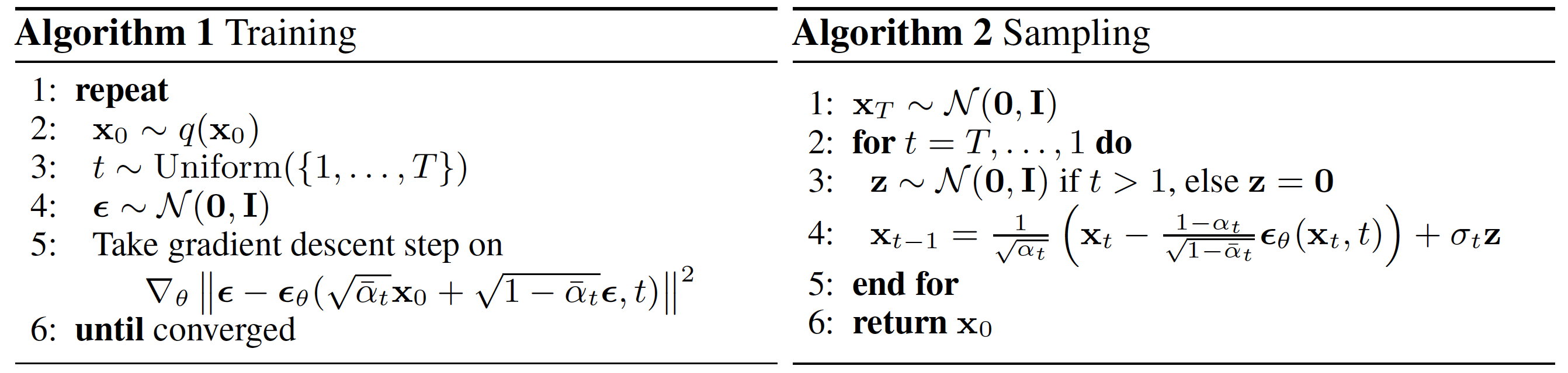
Training and Inference Algorithms. Adapted from [3].
Great YouTube tutorial by ExplainingAI really helped understand the whole concept!
References
Footnotes
\(k^N\) values if each RV can take \(k\) values↩︎
Two Gaussians with different variances, \(\mathcal{N}(\textbf{0}, \sigma_1^2\mathbb{I})\) and \(\mathcal{N}(\textbf{0}, \sigma_2^2\mathbb{I})\) can be merged to a new Gaussian distribution \(\mathcal{N}(\textbf{0}, (\sigma_1^2 + \sigma_2^2)\mathbb{I})\)↩︎
\(\mathcal{N}(\textbf{x}; \boldsymbol{\mu}, \boldsymbol{\sigma}^2) \propto \text{exp}(-\frac{1}{2} \frac{(\textbf{x} - \boldsymbol{\mu})^2}{\boldsymbol{\sigma}^2})\)↩︎
\(q(\textbf{x}_t | \textbf{x}_{t - 1}, \textbf{x}_0) = \frac{q(\textbf{x}_{t - 1} | \textbf{x}_t, \textbf{x}_0) \cdot q(\textbf{x}_t | \textbf{x}_0)}{q(\textbf{x}_{t - 1} | \textbf{x}_0)}\)↩︎
\(D_{KL}(p \parallel q) = \underset{x \sim p(x)}{\int} p(x) \log \frac{p(x)}{q(x)}\)↩︎
For two Gaussians with same covariance matrices \(p = \mathcal{N}(\textbf{x}; \boldsymbol{\mu}_1, \mathbf{\Sigma})\) and \(q = \mathcal{N}(\textbf{x}; \boldsymbol{\mu}_2, \mathbf{\Sigma})\), their \(D_{KL}(p \parallel q) = \frac{1}{2 \lVert \mathbf{\Sigma} \rVert^2_2} \lVert \boldsymbol{\mu}_1 - \boldsymbol{\mu}_2 \rVert^2\)↩︎