Convolution

For two functions \(f(x)\) and \(g(x)\), the convolution function \(f(x) * g(x)\) is defined as:

\[\begin{equation} (f * g) (t) = \int_{-\infty}^{\infty} f(τ) ⋅ g(t - τ) dτ \end{equation}\]

for discrete samples that we deal with: \[\begin{equation} y[n] = f[n] * g[n] = \sum_{k = -∞}^{∞} f[k] ⋅ g[n - k] \end{equation}\]

if \(f\) has \(N\) samples and \(g\) has \(M\) samples, then the convolved function has \(N + M - 1\) samples. A basic rule: “flip any one of the functions, overlap it with the stationary one, multiply and add, and then traverse over.”

import numpy as np
import matplotlib.pyplot as plt

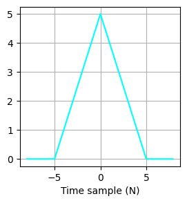
def triangle(x):
  if x >= 0 and x <= 5:
    return 5 - x
  elif x < 0 and x >= -5:
    return 5 + x
  else:
    return 0

def rect(x):
  if -5 <= x <= 5:
    return 5
  return 0

def signal(f, x):
  return [f(i) for i in x]

x = np.arange(-8, 8, 0.1)
f_x = signal(rect, x)
plt.plot(x, f_x, color = "black")
plt.xlabel("Time sample (N)")
plt.grid()
plt.show()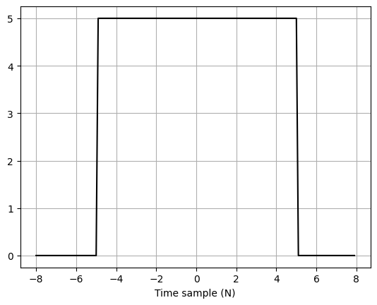

\(O(N^2)\) complexity algorithm total \((N + M - 1) \cdot M\) or \((N + M - 1) \cdot N\) computations

A_signal, B_kernel = signal(rect, x), signal(rect, x)
N_signal, M_kernel = len(A_signal), len(B_kernel)
Y = np.zeros(N_signal + M_kernel - 1)
for i in range(len(Y)):
  for j in range(M_kernel):
    if i - j >= 0 and i - j < N_signal:
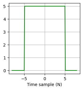
      Y[i] += A_signal[i - j] * B_kernel[j]

Convolution of two rect(\(x\))

plt.figure(figsize = (3, 3))
plt.plot(x, A_signal, color = "green")
plt.xlabel("Time sample (N)")
plt.grid()
plt.show()

plt.figure(figsize = (3, 3))
plt.plot(x, A_signal, color = "green")
plt.xlabel("Time sample (N)")
plt.grid()
plt.show()

print(f"Signal Length: {N_signal}, Convolved Signal Lenght: {len(Y)}")
plt.plot(Y, color = "red")
plt.xlabel("Index Number (k)")
plt.grid()
plt.show()

Signal Length: 160, Convolved Signal Lenght: 319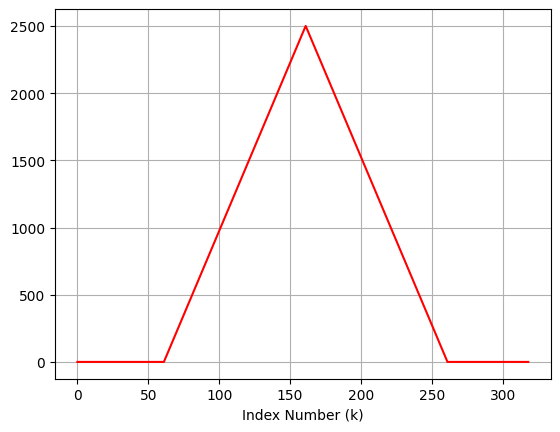

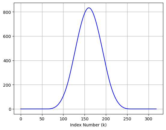
A_signal, B_kernel = signal(triangle, x), signal(triangle, x)
N_signal, M_kernel = len(A_signal), len(B_kernel)
Y = np.zeros(N_signal + M_kernel - 1)
for i in range(len(Y)):
  for j in range(M_kernel):
    if i - j >= 0 and i - j < N_signal:
      Y[i] += A_signal[i - j] * B_kernel[j]

Convolution of two triangle(\(x\))

plt.figure(figsize = (3, 3))
plt.plot(x, A_signal, color = "cyan")
plt.xlabel("Time sample (N)")
plt.grid()
plt.show()

plt.figure(figsize = (3, 3))
plt.plot(x, A_signal, color = "cyan")
plt.xlabel("Time sample (N)")
plt.grid()
plt.show()

print(f"Signal Length: {N_signal}, Convolved Signal Lenght: {len(Y)}")
plt.plot(Y, color = "blue")
plt.xlabel("Index Number (k)")
plt.grid()
plt.show()

Signal Length: 160, Convolved Signal Lenght: 319